Rethink LoRA initialisations for faster convergence

What is LoRA

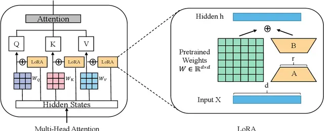
LoRA has been a tremendous tool in the world of fine tuning, especially parameter efficient fine tuning. It is an easy way to fine tune your models with very little memory requirements. LoRA was first introduced in this paper by Hu et al. The premise of LoRA is, upon fine tuning, the change in weights of the matrices are of low rank in comparison with the original matrix To exploit this, LoRA adds an adapter which we can train while having the initial model weights frozen. $$ W’ = W + \Delta W = W + AB \space\space where \space\space A=\mathbb{R}^{(m,r)}, \space\space B=\mathbb{R}^{(r,n)}, \space\space W=\mathbb{R}^{(m,n)}$$ Here W are the initial weights and ΔW is the change in weights upon fine tuning. The advantage with LoRA unlike other PEFT techniques is that LoRA weights can be merged back into the initial model and hence there will not be any performance loss at inference. Also, because this is just an adapter, one can dynamically switch between adapters and having no adapter aka using base model. Such versatility and flexibility propelled LoRA to become the most used PEFT technique and the best part is, this is model agnostic. So any model that has linear layers, can use this. It has been very famous in both Image generation and NLP worlds off late.

LoRA Initialization

Now comes the question. If we add another weight to existing weight matrix, wouldn’t it put the model off? Yes, adding any random stuff does impact the model quality. But to ensure that at initialisation model doesn’t suffer from such issues, we initialise matrices A and B such that the product ΔW = AB = 0.

But how do you do that? Initialising both to zero is a viable option but would inhibit the model from learning. So the original paper proposes to initialise A with kaiming uniform (just uniform initialisation with differnt range parameter). So problem solved right? We now have a non zero A and a zero B such that AB = 0. Well technically yes and this has been working for long. So why change it huh?

Well I wasn’t really satisified with this. I thought, why not try out some different initialisations? But the trick here is to also ensure that our initialisation follows AB = 0. So thoughts come to your mind? The first and easiest one is to reverse the initialisations aka setting A = 0 and B = kaiming_uniform.

If you take the example of llama-3-8B, here’s how the model looks like after injecting LoRA adapters of rank 8

(layers): ModuleList(
  (0-31): 32 x LlamaDecoderLayer(
    (self_attn): LlamaSdpaAttention(
      (q_proj): lora.Linear(
        (base_layer): Linear(in_features=4096, out_features=4096, bias=False)
        (lora_A): ModuleDict(
          (default): Linear(in_features=4096, out_features=8, bias=False)
        )
        (lora_B): ModuleDict(
          (default): Linear(in_features=8, out_features=4096, bias=False)
        )
      )
      (k_proj): lora.Linear(
        (base_layer): Linear(in_features=4096, out_features=1024, bias=False)
        (lora_A): ModuleDict(
          (default): Linear(in_features=4096, out_features=8, bias=False)
        )
        (lora_B): ModuleDict(
          (default): Linear(in_features=8, out_features=1024, bias=False)
        )
      )
      (v_proj): lora.Linear(
        (base_layer): Linear(in_features=4096, out_features=1024, bias=False)
        (lora_A): ModuleDict(
          (default): Linear(in_features=4096, out_features=8, bias=False)
        )
        (lora_B): ModuleDict(
          (default): Linear(in_features=8, out_features=1024, bias=False)
        )
      )
      (o_proj): lora.Linear(
        (base_layer): Linear(in_features=4096, out_features=4096, bias=False)
        (lora_A): ModuleDict(
          (default): Linear(in_features=4096, out_features=8, bias=False)
        )
        (lora_B): ModuleDict(
          (default): Linear(in_features=8, out_features=4096, bias=False)
        )
      )
      (rotary_emb): LlamaRotaryEmbedding()
    )
    (mlp): LlamaMLP(
      (gate_proj): lora.Linear(
        (base_layer): Linear(in_features=4096, out_features=14336, bias=False)
        (lora_A): ModuleDict(
          (default): Linear(in_features=4096, out_features=8, bias=False)
        )
        (lora_B): ModuleDict(
          (default): Linear(in_features=8, out_features=14336, bias=False)
        )
      )
      (up_proj): lora.Linear(
        (base_layer): Linear(in_features=4096, out_features=14336, bias=False)
        (lora_A): ModuleDict(
          (default): Linear(in_features=4096, out_features=8, bias=False)
        )
        (lora_B): ModuleDict(
          (default): Linear(in_features=8, out_features=14336, bias=False)
        )
      )
      (down_proj): lora.Linear(
        (base_layer): Linear(in_features=14336, out_features=4096, bias=False)
        (lora_A): ModuleDict(
          (default): Linear(in_features=14336, out_features=8, bias=False)
        )
        (lora_B): ModuleDict(
          (default): Linear(in_features=8, out_features=4096, bias=False)
        )
      )
    )
  )
)
Note: truncated for better readability

Reversing Initialization

As you see, for a given layer (0-31), LoRA A and B would have same parameters in q_proj (query matrix), k_proj (key matrix), and o_proj. LoRA A has more parameters in v_proj(value matrix). LoRA B has more paramters in gate_proj and up_proj. Generally MLPs in Transformer have bigger hidden dimension than any other layers. So without loss of generality, B matrix has more paramters than A. So if nothing else, it ameks sense to initialise B with kaiming uniform and A with zeros. This is one of the things I tried.

Orthogonal initialisation

Two vectors are called orthogonal when their dot product is zero. So in our use case, we need a lot of such orthogonal vectors. Those should be orthogonal in 8-D space (or whatever the lora rank is). And we need m such vectors in A and n such vectors in B. If we say have a few orthogonal vectors, any linear combinations of those would be orthogonal too.

say vectors \( {v_1, v_2, v_3, \ldots v_x} \) are set of orthogonal vectors which means, \( v_i.v_j = 0 \space \forall \space i,j \) so for any linear combination
$$ C_a = a_1 v_1 + a_2 v_2 + \ldots a_x v_x $$ $$ C_b = b_1 v_1 + b_2 v_2 + \ldots a_x v_x $$ So the dot product would be (assuming $v_i$ is unit vector) $$ C_a.C_b = (a_1 v_1 + a_2 v_2 + \ldots a_x v_x).(b_1 v_1 + b_2 v_2 + \ldots a_x v_x) $$ $$ = \sum_{i} a_ib_iv_i^2 + \left[ \sum_{i}\sum_{j\neq i} a_ib_j(v_iv_j) = 0 \right] = \sum_{i} a_ib_i$$

Note that if we ensure that either of \(a_i\) or \(b_i\) is zero, the product would be exact zero. For that, if we make sure that if a vector is in \(C_a\) the same vector isn’t in \(C_b\), we’d have \(C_a.C_b = 0\)

Now the task boils down to finding a few orthogonal. There are two methods I can think of for this.

1. Create a random matrix. Find orthogonal decomposition of it. The rows of the matrix would be orthogonal.
2. Take random linear combinations of rows of Identity matrix. They would be orthogonal too.

So, take those r linear combinations, split into two groups. First group would have some r/2 of those vectors and the second group would have the remaining r/2 vectors. From each set, we can create a matrix by linearly combining the elements of that set only.

To create set of random linear combinations, we can simply create a random matrix and multiply it with the matrix created by those corresponding sets.

with torch.no_grad(): #Ensure that the gradients aren't tracked
    # Method 1: QR decomposition of a random matrix
    X = torch.randn(r, r)
    Q, _ = torch.linalg.qr(X)
    
    # Method 2: Just use identity matrix's columns
    Q = torch.eye(r, r)

    set1 = Q[0::2,:]  # Odd rows
    set2 = Q[1::2,:]  # Even rows

    a_wt = torch.randn(m, r//2).mm(set1).to(torch.bfloat16).T/10.0
    b_wt = torch.randn(r//2, n).T.mm(set2).to(torch.bfloat16)/10.0

if init_lora_weights is True:
    # Contiguous cuz for saving the weights to disk after n steps, we need them to be contiguous
    self.lora_A[adapter_name].weight = nn.Parameter(a_wt.contiguous())
    self.lora_B[adapter_name].weight = nn.Parameter(b_wt.contiguous())

The only problem with Method 2 where we use Identity matrix is, after splitting into two sets of size (r, r/2), there are some vectors where r/2 of those values are zero. Hence half the rows of A and half the columns of B are zero which is a bummer.

Note: If you have any other different ideas for initialisation, feel free to reach out to me and we can discuss.

Results

Ok enough of theory. How does it hold in practice? Well I’ve tried training LoRAs with models of different sizes and architectures. The results look promising. Here’s the wandb project where I’ve been tracking my runs and here’s the wandb report of the same

I ran my experiemnts on four different models namely llama-2-7B, llama-2-13B, llama3-8B and mistral-7b-v0.3. The datasets I used are MetaMathQA and MagicCoder-evol 10k and 100k variants. I used the same train and eval samples for each of the models. Other parameters I used for the training

lora_r = 8
learning_rate = 1e-4
target_modules = ['down_proj','up_proj','gate_proj','q_proj','k_proj','v_proj','o_proj'] (every module)
random_seed = 42 (same for CUDA)
warmup_steps=0.02,
max_grad_norm=0.3,
optim=f"paged_adamw_32bit",

Note: I’m only tracking eval loss and performance on downstream tasks is a thing for another day :)

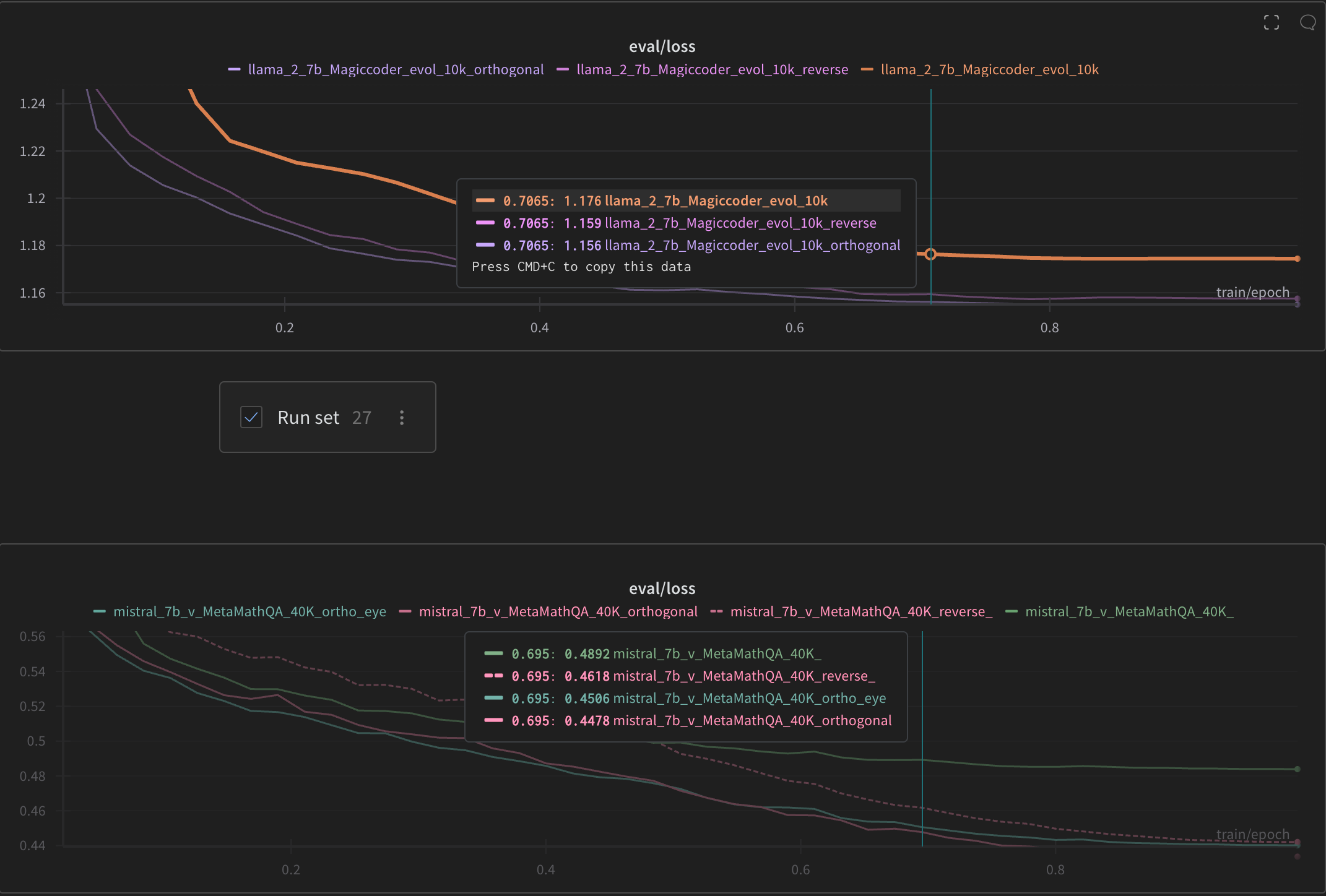
wandb render of the same

If you observe, reverse initialisation definitely outperforms the normal initialisation. And most of the cases, orthogonal initialisation outperforms both the normal initialisation and the reverse initialisation.

So for no loss, we’re improving the convergence of LoRA. I know it takes a little time to initialise all the matrices given that we’re doing QR decomposition for each of the layers. But this is a one time thing in the whole training cycle. It definitely makes sense to consider this as a starting point for initalisations.

Analysis and Bonus content

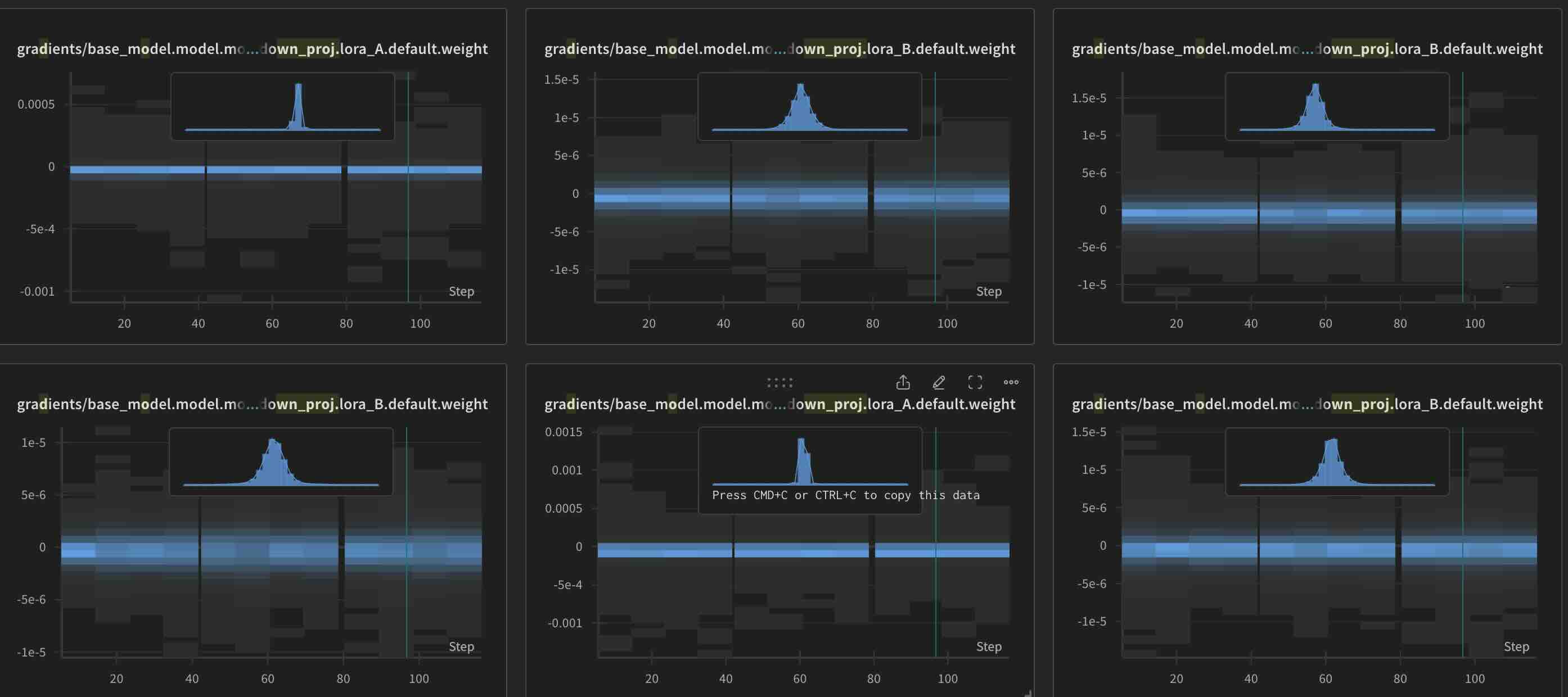
One other interesting thing I observed while training is the gradients. Thanks to wandb, I was able to track the gradeints. What I observed is, irrespective of initialisation, gradients for LoRA B are always greater than those of LoRA A. This is something we might need to look into later…

Gradients for Normal initialisation 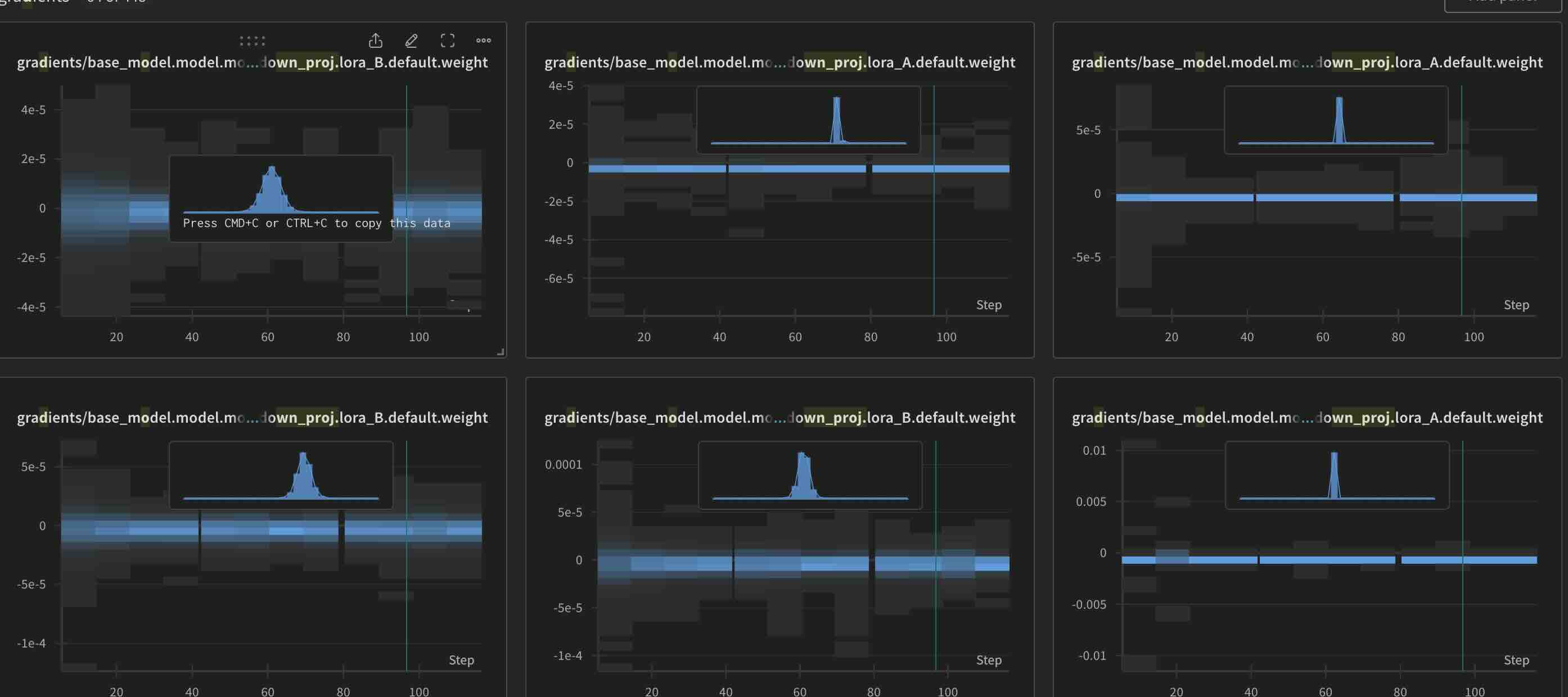Gradients for Reverse initialisation Gradients for Orthogonal initialisation

What does this all tell us? If you ask me, there are some things that we can infer or take away from this

1. The gradeints hint us towards having separate learning rates for A and B matrices.
2. Different initalisations for LoRA should be further experimented upon. There are improvements we can harness.
3. We probably need more ablation studies for newer techniques. Someday maybe even scaling laws for LoRA (or PEFT in general).

Thanks for the read :) If you have any questions, comments, suggestions please feel free to reach out to me. Cheers …