Exploring the Mixture of Experts

Mixture of Experts

Introduction

Previously we have talked about Transformer and attention being re-imagined from the first principles. While that gives a very good understanding of how transformers work, specifically the attention mechanism, there has been a lot of progress ever since. One of the under-represented parts of the transformer is the FFNN. MoE or mixture of experts is a natural continuation of the same. Today we’ll try to reimagine the same.

FFNN

Let’s start with the FFN. Attention is all cool but attention doesn’t mix features with one another. It only brings you the information from the other tokens so get a context of what you’re surrounded by thus giving you an idea of what you potentially are. But the model also needs to know which features of the token are important and which are potentially discardable given the context. This is pretty much the job of FFNN. Here we try to separate the features of interest from the non-interesting features. Given a token and its features, we project it from the model dimension to a higher dimension called the MLP dimension, or intermediate size, and apply a nonlinearity element-wise to achieve that. In the recent past, we have Gated Linear unit as the buiding block which goes as follows:

\[\begin{aligned} X &\in \mathbb{R}^{n \times d} \\ W_{up}, W_{gate} &\in \mathbb{R}^{d \times d_{mlp}} \\ W_{down} &\in \mathbb{R}^{d_{mlp} \times d} \\ \\ g &= X @ W_{gate} \quad \in \mathbb{R}^{n \times d_{mlp}} \\ u &= X @ W_{up} \quad \in \mathbb{R}^{n \times d_{mlp}} \\ s &= \text{SiLU}(g) \\ gu &= s \odot u \\ \text{MLP}(X) &= gu @ W_{down} \quad \in \mathbb{R}^{n \times d} \end{aligned}\]

For more information on how FFNN works, please refer to this section in our previous blog.

The motivation for MoE

If you notice closely, the non linearity used in general is SiLU or ReLU or GeLU. All of which pretty much set almost half the input values (negative ones) to zero.

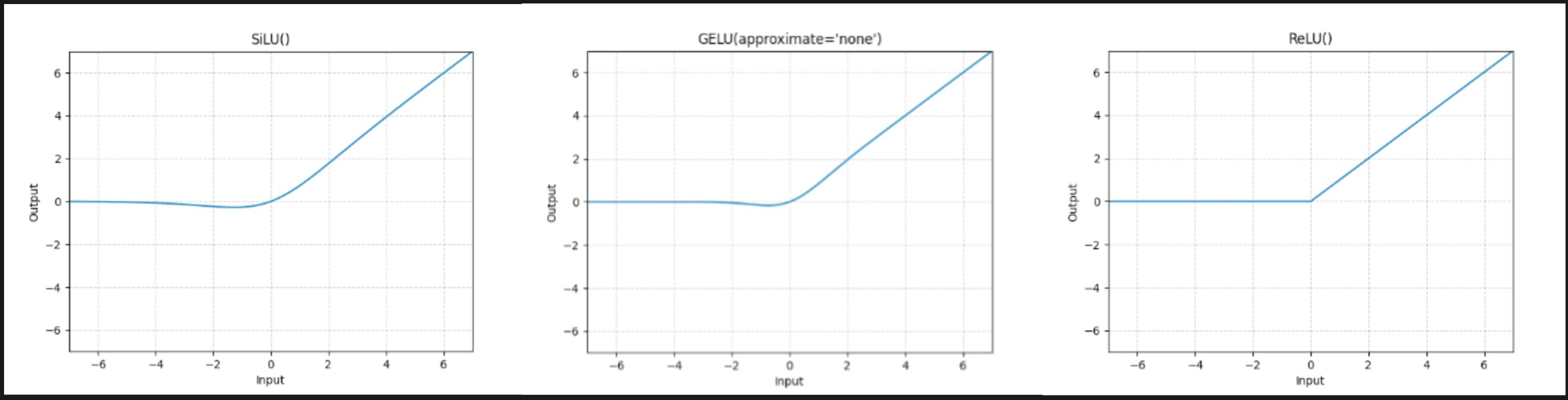FFNN Activations

After computing the gate proj we just basically throw away the corresponding features. Up proj being an element wise product with the output after the activation, wouldn’t change the feature from 0. So we are potentially computing a lot of features which are not useful. What if we can avoid that? Yeah we would like to solve exactly that problem. We would like to know which columns of the MLP matrix are useful for us and which are not. But how do we know which ones to avoid? Ideally it should depend on your hidden state just before the MLP.

The simplest way to do it is to have a linear projection(yeah like always) that predicts the importance of a column for the given input. So for an input $X \in \mathbb{R}^{d}$ (single token), we need a matrix that takes d features and outputs us $d_{mlp}$ values. But that would be a $\mathbb{R}^{d \times d_{mlp}}$ matrix. So by doing this we’re literally repeating the computation we’d have done for gate_proj.

The input dimension cannot be compromised on. What can be changeed is the output dimension. What does it mean to the operations? Essentially we find a smaller dimension, say n, such that we predict n values per input and then use those values to pick some of the $d_{mlp}$ columns. But we should be careful as to not involve any more non simple, non trivial transformations on the said n that adds to the compute and parameter cost. When tasked with such constraints, always try to pick the simplest way out. So instead of having to take a decision for each of the columns, what if we take a single decision for a group of columns? This essentially is equivalent to saying, “Let us group $d_{mlp}$ columns into $k$ buckets, and for each bucket we decide whether to use it or not”.

Lets see how (much) that reduces our compute. If we multiply a matrix of shape (m,k) with another matrix of shape (k,n) to get an output of shape (m,n), we’re doing O(mnk) computations. You can visualise this by taking the perspective of the ouptut. For each of the values in the output, we need to do a dot product between vectors of size k. So we do k multiplications and k-1 additions (of k numbers). And we have m*n such values. So the total computation is O(mnk). If you consider addition and multiplication as 1 operation, we’re looking at ~2mnk ops. Please excuse the abuse of O notation here :).

So initially for s tokens, to perform full computation (MLP), we have:

\[\begin{aligned} g &= X W_{\text{gate}} &&\in \mathbb{R}^{s \times d_{\text{mlp}}} &&\;\; \mathcal{O}(s\, d\, d_{\text{mlp}}) \\ u &= X W_{\text{up}} &&\in \mathbb{R}^{s \times d_{\text{mlp}}} &&\;\; \mathcal{O}(s\, d\, d_{\text{mlp}}) \\ s' &= \mathrm{SiLU}(g) && &&\;\; \mathcal{O}(s\, d_{\text{mlp}}) \\ gu &= s' \odot u &&\in \mathbb{R}^{s \times d_{\text{mlp}}} &&\;\; \mathcal{O}(s\, d_{\text{mlp}}) \\ \text{out} &= gu W_{\text{down}} &&\in \mathbb{R}^{s \times d} &&\;\; \mathcal{O}(s\, d\, d_{\text{mlp}}) \end{aligned}\] \[\text{total} \;\approx\; 3\,\mathcal{O}(s\, d\, d_{\text{mlp}}) \quad\text{(matmuls dominate)}\]

---

In the latter case, we have weights of the following shapes, with n experts each outputting (d_e) features:

\[d_e = \frac{d_{\text{mlp}}}{n} \quad \text{and} \quad W'_{\text{up}} \in \mathbb{R}^{n \times d \times d_e} \quad W'_{\text{gate}} \in \mathbb{R}^{n \times d \times d_e} \quad W'_{\text{down}} \in \mathbb{R}^{n \times d_e \times d} \quad W'_{\text{picker}} \in \mathbb{R}^{d \times n} \quad\]

First we compute preference scores, find top-k, and pick the corresponding k experts with the flop count:

\[\begin{aligned} \text{scores} &= X W'_{\text{picker}} &&\in \mathbb{R}^{s \times n} &&\;\; \mathcal{O}(s\, d\, n) \\ \text{TopK} &= \mathrm{top}_k(\text{scores}) &&\in \mathbb{R}^{s \times k} &&\;\; \mathcal{O}(s\, n \log k) \\ g &= X\, W'_{\text{gate}}[\text{TopK}] &&\in \mathbb{R}^{s \times (k d_e)} &&\;\; \mathcal{O}(s\, d\, k\, d_e) \\ u &= X\, W'_{\text{up}}[\text{TopK}] &&\in \mathbb{R}^{s \times (k d_e)} &&\;\; \mathcal{O}(s\, d\, k\, d_e) \\ s' &= \mathrm{SiLU}(g) && &&\;\; \mathcal{O}(s\, k\, d_e) \\ gu &= s' \odot u &&\in \mathbb{R}^{s \times (k d_e)} &&\;\; \mathcal{O}(s\, k\, d_e) \\ \text{out} &= gu\, W'_{\text{down}}[\text{TopK}] &&\in \mathbb{R}^{s \times d} &&\;\; \mathcal{O}(s\, d\, k\, d_e) \\ \text{result} &= \sum_{i \in \text{TopK}} \text{out}_i \,\odot\, \text{scores}_i &&\in \mathbb{R}^{s \times d} &&\;\; \mathcal{O}(s\, d\, k) \end{aligned}\] \[\text{total ops} = \mathcal{O}(s\, d\, k\, d_e) + \mathcal{O}(s\, d\, n) + \mathcal{O}(s\, n \log k)\]

Comparing the two:

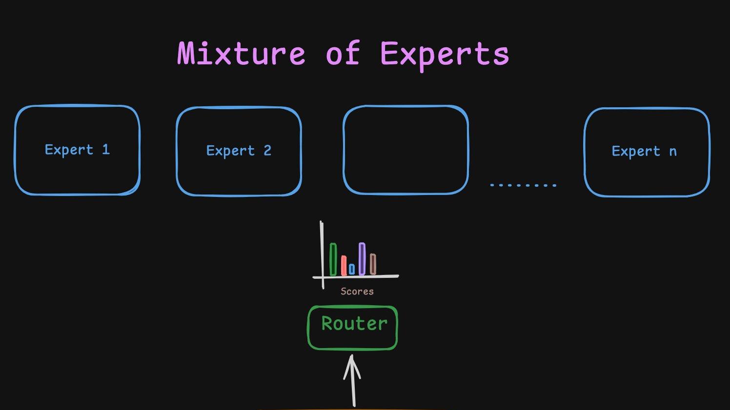
\[\begin{aligned} \mathrm{Ops}_{\text{MLP}} &= \mathcal{O}(s\, d\, d_{\text{mlp}}) \\ \mathrm{Ops}_{\text{MoE}} &= \mathcal{O}(s\, d\, k\, d_e) + \mathcal{O}(s\, d\, n) + \mathcal{O}(s\, n \log k) \\ &= \mathcal{O}\!\left(s\, d\, k\, \frac{d_{\text{mlp}}}{n}\right) + \mathcal{O}(s\, d\, n) + \mathcal{O}(s\, n \log k) \end{aligned}\]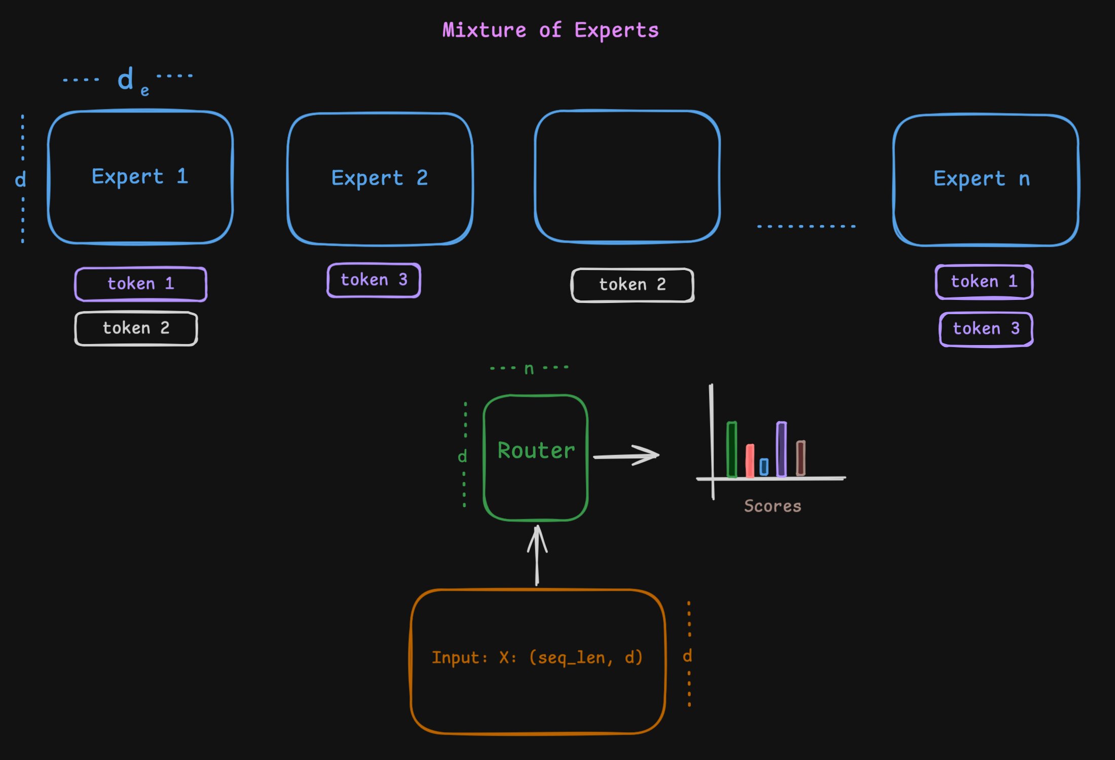

MoE visualised

---

Of course a lot hinges on the ratio between (k) and (n). From a hardware and performance standpoint, it relies on parallelising the chosen (k) experts efficiently.

I’d leave it to you to compare these for typical MoE configs like Qwen3-30B-A3B or GPT OSS 20B and verify for yourself that this makes sense mathematically.

For the lazy reader, here’s the math (click to expand)

1. Qwen3-30B-A3B

From the config:

• $d = 2048$ (hidden_size)
• $n = 128$ (num_experts)
• $k = 8$ (num_experts_per_tok)
• $d_e = 768$ (moe_intermediate_size)

Equivalent dense intermediate size: $d_{\text{mlp}} = n d_e = 128 \cdot 768 = 98304$.

• Dense ops (dominant matmuls):
  $3 \cdot s\, d\, d_{\text{mlp}} \approx 3 \cdot s \cdot 2048 \cdot 98304$
• MoE ops:
  • Routing: $s\, d\, n = s \cdot 2048 \cdot 128$
  • Experts: $3 \cdot s\, d\, k\, d_e = 3 \cdot s \cdot 2048 \cdot 8 \cdot 768$

That is a $\sim93.7\%$ reduction in FFN FLOPs against the naive dense layer counterpart!

2. GPT OSS 20B

From the config:

• $d = 2880$ (hidden_size)
• $n = 32$ (num_local_experts)
• $k = 4$ (num_experts_per_tok)
• $d_e = 2880$ (intermediate_size per expert)

Equivalent dense intermediate size: $d_{\text{mlp}} = n d_e = 32 \cdot 2880 = 92160$.

• Dense ops (dominant matmuls):
  $3 \cdot s\, d\, d_{\text{mlp}} \approx 3 \cdot s \cdot 2880 \cdot 92160$
• MoE ops:
  • Routing: $s\, d\, n = s \cdot 2880 \cdot 32$
  • Experts: $3 \cdot s\, d\, k\, d_e = 3 \cdot s \cdot 2880 \cdot 4 \cdot 2880$

This yields a $\sim87.5\%$ compute reduction in the FFN block while retaining a massive $92$K parameter width per token routing!

Consolidation

This is how the output is calculated for the MoE. out[i] is the output of the ith expert. We multiply by the scores to respect the preferences of the tokens.

\[\begin{aligned} \text{scores} &= X @ W_{router} \\ \text{out}[i] &= (\text{SiLU}(X \cdot W_{gate}[i]) * (X\cdot W_{up}[i])) \cdot W_{down}[i] \quad \in \mathbb{R}^{d} \quad | \quad \mathcal{O}(d \cdot k) \\ \text{out} &= \sum_{i \in \text{TopK}} \text{scores}[i] \cdot \text{out}[i] \quad \in \mathbb{R}^{d} \quad | \quad \mathcal{O}(d \cdot k) \end{aligned}\]

Training

Inference is straightforward. You have a token; you get the preference scores for each of the buckets, called experts, and pick the top few among them to pass the activations through those experts. Sweet and simple. One should ideally forward pass through all the chosen k experts parallelly.

For trainig, you have s tokens instead of 1 like we discussed above. Each token has its own k preferred experts among the n. So the task becomes more tricky to first calculate the router scores, find out top-k per token, then somehow pass the set of appropriate tokens for each expert. pytorch has an operation to do all this parallelly called torch._grouped_mm. We also made LoRA training on MoE more efficient at Unsloth. Check out here.

One caveat we’ve been brushing under the rug so far, what if an expert is not chosen by any token? It is not involved in the forward pass, hence wouldn’t be involved in the backward pass either. So it gets no chance to get better to be potentially be preferred by tokens in the future. This is a vicious cycle. So expert utilisation being (approximately) uniform is an important thing. There are a few ways to enfoce this.

We will talk about these more at a later time. For now we just introduce the ideas to the curious minds.

Auxiliary Loss

Most of the MoE works add an auxiliary loss to the main loss. This loss is calculated on the router scores and is used to encourage the router to distribute the tokens evenly among the experts. One in theory can compare the router’s current distribution to the uniform distribution and add a difference as a loss.

But there’s a small problem with adding such a bias. Natural language potentially has a long tail. Some experts might be specialising in certain domains. Forcing a generic language expert to be used as much as the “coding” expert or “math” expert might not be a good idea.

Router Bias

Deepseek V3 again famously implemented this to counteract the imbalance. Instead of adding an auxiliary loss, we modify the router scores so that we reduce the scores of the routers that are heavily being picked historically while increasing the ones that are not picked much.

\[\begin{aligned} \text{scores} &= \text{scores} + \text{bias} \\ e_i &= \text{number of tokens expert i sees} = \sum_{j=1}^{s} \mathbb{I}(i \in \text{TopK}(j)) \\ \bar{e} &= \text{expected number of tokens per expert} = \frac{s}{n} \\ b_i &= b_{i-1} + \lambda \cdot \text{sign}(e_i - \bar{e}) \\ \end{aligned}\]

Expert choice

So far we’ve been talking about tokens picking experts which might lead to imbalance. But what if we flip the problem on its head? What if we let the experts pick the tokens? This is called expert choice routing famously used in Llama 4 family of models.

Each expert has its own ranking mechanism and picks only the top-k among the many tokens. But this has a serious flaw hiding underneath. This breaks causality. In token choice, each token is independently routed to experts irrespective of the existence of other tokens. Here though it is different. Lets see a small example.

Assume each expert picks only 1 token. If expert 1 prefers token a over token b, then in presence of both the tokens, expert 1 will pick a. But if a is not present expert 1 will pick b. So essentially we’re leaking information to b whether a is present in the sequence or not. Leaking because, b can be earlier in the sequence than a. This breaks causality. Perhaps potentially (among the many reasons) why llama 4 is not up to the mark.

Shared Expert

Some models use a shared expert which is used by all the tokens. This is done to make sure that common knowledge is shared across all the tokens and there is no contention to choose between a common knowledge expert and a specialized expert.

\[\begin{aligned} scores &= X @ W_{router} \\ gate_i &= SiLU(X \cdot W_{gate}[i]) \quad up_i = X \cdot W_{up}[i] \\ gate_{shared} &= SiLU(X \cdot W_{gate_{shared}}) \quad up_{shared} = X \cdot W_{up_{shared}} \\ out[i] &= (gate_i * up_i) \cdot W_{down}[i] \\ out_{shared} &= (gate_{shared} * up_{shared}) \cdot W_{down_{shared}} \\ out &= out_{shared} + \sum_{i \in \text{TopK}} scores[i] \cdot out[i] \end{aligned}\]

Do note that for some models there are more than one shared expert. The resulting equation looks exactly like that of the “routed” experts but every token goes through all of the said “shared” experts. You get the idea.

Parallelism in MoE: Expert Parallelism

So in a previous blog, we have talked about parallelism strategies and how they can be applied to Transformers, both attention and MLP. MoE is no exception to this. It offers us more flexibility in terms of parallelism strategies.

One thing we need to ensure when parallelising things is to minimise communication as much as possible. Because the time you spend communicating is the time you are not computing for the most part.

One can place different experts (or different groups of experts) onto different GPUs to reduce the memory pressure on single GPU either to parallelise MoE for throughput gains or due to memory constriants on single GPU. This is called expert parallelism. The number of GPUs you split the experts across is called expert parallelism degree.

When you do expert parallelism, you can either replicate the attention modules across the expert parallelism degree or you can split them and use tensor parallelism as discussed in the previous blog. It all boils down to your GPU capacity. If you choose to replicate the attention modules, you are pretty much doing Data Parallel across GPUs for the attention modules. Then you can distribute the tokens to the corresponding GPUs according to their choice of experts. Once the computation is done, you can gather your share of tokens from all the GPUs and then go ahead with your own stuff for the later computations.

Now that you know expert parallelism exists, do you see why the token distribution being uniform is crucial even from a performance standpoint? Uniform distribution ensures all the experts compute their share together parallelly and there’s not time wasted waiting for an expert’s computation. It all fits well.

Note that because this happens for every layer, I wouldn’t think it is a smart idea to parallelise this across nodes. This is great for parallelising within a node across the GPUs which are connected by high speed bandwidth like PCIe or NVLink.

Below is an image showing how expert parallelism works. Note that tokens are color coded to corresponding GPUs. Also there is definite imbalance in the load that each GPU is bearing.

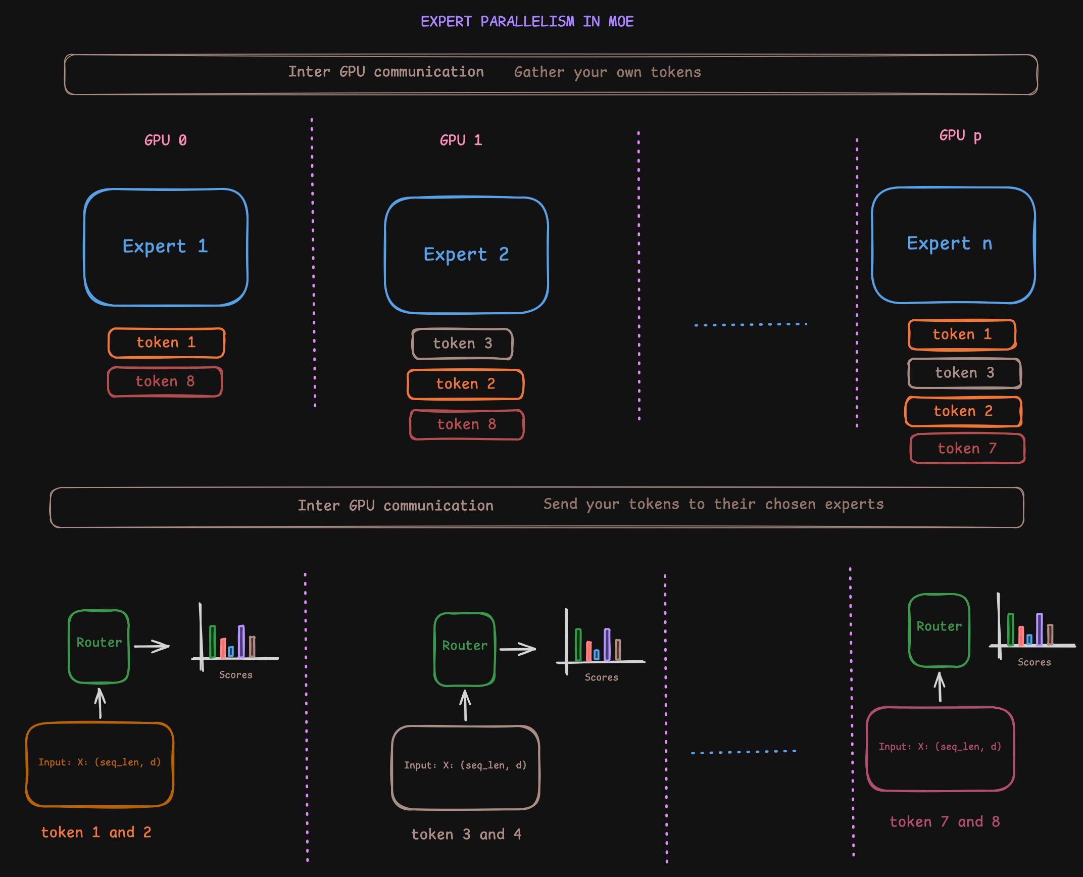Expert parallelism (note that tokens are color coded to corresponding GPUs)

So why go through all this hassle?

So why go through all this hassle if it doesn’t translate to any gains right? But there is a lot to be gained here. At decode time, we’re only activating k out of the n experts. So we’re saving on a lot of compute and memory bandwidth thus saving us inference time. Note that we haven’t sacrificed any of the model’s capacity. We’ve just made it smartly choose what it needs to use. At inference time, it is equivalent compute to that of a model with much fewer parameters.

In traditional terminology, because you are hitting/activating only k out of the n experts, you count the number of parameters you touch in the path as the effective number of parameters often called as Activated Parameters.

When you see a model name like unsloth/Qwen3-30B-A3B-Instruct-2507, the total number of parameters, 30B, is followed by the number of activated parameters, A3B. So only 3B parameters are activated per token. Pretty cool huh!

Some more details

Quick math

So let’s do a quick math. If a model is said to have k experts, n activated and is total of T parameters while A are activated, $n_l$ is total number of layers, where #X denotes number of parameters in module X, we have:

\[\begin{aligned} \#lm\_head + \#attention \cdot n_l + \#moe \cdot n_l &+ \#router \cdot n_l + \#embedding = T \\ \#lm\_head + \#attention \cdot n_l + \#moe \cdot \frac{n}{k} \cdot n_l &+ \#router \cdot n_l + \#embedding = A \\ \implies \left(1-\frac{n}{k}\right)\#moe \cdot n_l &= T - A \\ \implies \#moe &= \frac{T-A}{\left(1-\frac{n}{k}\right)\cdot n_l} \end{aligned}\]

We still have to take a lot of decisions here. What is the optimal k and n? Typically in the earlier works a ratio of 1:8 was used for k:n. But recent works have shown that we can do better. For a fixed number of total parameters and activated paramters, the sparser you choose the better aka lower k and higher n. This is why you see 128, 256 and even 512 experts in recent times.

We just briefly touched upon load balancing but it is a deep topic in itself. Sometimes, when an expert is overwhelmed with tokens, some tokens are dropped to avoid going over the capacity and potentially causing OOMs or just general slowdown.

Sometimes (albeit not a lot), instead of training MoE from scratch, what people (read: Mixtral) do is take a pre-trained dense model and convert it into an MoE model. They do this by replicating the MLP layers and then replacing the original MLP layer with a router and the replicated layers. So the attention weights and the MLP weights are from previously trained dense model and router takes care of dynamically routing the tokens to new “expert” MLPs.

One mroe thing to note is that not all layers need to be MoE. There are some models that mix and match both like the GLM-4.7-Flash.

Outro

With this I leave you with a good motivation to appreciate MoE and what they bring to the table. Also a little understanding of the challenges of training and serving them and how to tackle those. We will go into more details in future blogs. Thanks for reading thus far. If you have any comments, concerns, questions, or suggestions, please feel free to reach out to me. You can find me on LinkedIn or Twitter. I’ll leave it here for now. Sayonara :)