The MathemaTricks behind FlashAttention

Introduction

In Attention and Transformers, Imagined, we built up the idea of attention from first principles. As a quick refresher, given a sequence of tokens, we compute query, key, and value matrices, and the final attention output is

\[O = \operatorname{softmax}\left(\frac{QK^\top}{\sqrt{d}}\right)V\] \[Q, K, V \in \mathbb{R}^{n \times d}\]

If you write it out step by step in PyTorch, it looks roughly like this:

import math
import torch

def attention(Q, K, V):
    attn_scores = torch.matmul(Q, K.transpose(-2, -1))  # [n, d] @ [d, n] = [n, n]
    attn_probs = torch.softmax(attn_scores / math.sqrt(Q.shape[-1]), dim=-1)  # [n, n]
    output = torch.matmul(attn_probs, V)  # [n, n] @ [n, d] = [n, d]
    return output

For smaller values of $n$, this is perfectly fine. But as $n$ grows, the intermediate attention score matrix, and often the probability matrix too in a naive implementation, put enormous pressure on GPU memory. With context lengths growing and workloads like coding or reasoning demanding longer traces, this quickly becomes a bottleneck.

Take a 128K sequence as an example:

\[n = 128 \times 1024 = 131072\] \[\operatorname{attn\_scores} = QK^\top \in \mathbb{R}^{n \times n}\] \[n^2 = 17{,}179{,}869{,}184 \text{ elements per head}\] \[2n^2 = 34{,}359{,}738{,}368 \text{ bytes} \approx 32 \text{ GiB per head in BF16}\]

If you have multi-head attention, this cost multiplies across heads. So even at 128K, a single head wants roughly 32 GiB just to hold the attention scores, which is already more than many GPUs can fit comfortably.

This is what people mean when they say attention is quadratic in sequence length.

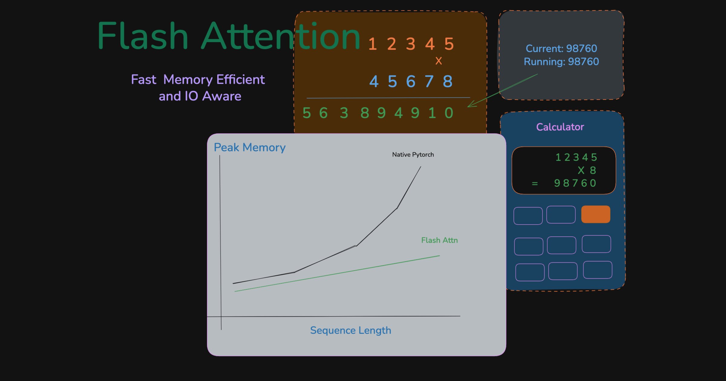
The calculator analogy

Imagine multiplying two large numbers with a calculator that can only add or multiply single digits. You also have a sheet of paper for writing results and a small scratchpad for intermediate work. Assume you cannot do any mental math. The paper is larger than the scratchpad, but it is still limited.

There are two ways to do this. The naive approach is standard long multiplication: write each intermediate row to paper, shift it, and add everything at the end. If each number has $n$ digits, you end up writing on the order of $n^2$ digit slots. As the numbers grow, you can quickly run out of room on the paper. But do you really need to store every intermediate row on paper?

Naive multiplication: write every intermediate row to paper.

One smarter approach is to keep a running total on the scratchpad. You copy the first number, process one digit of the second number at a time, and immediately merge that contribution into the running sum. At any point, the scratchpad only needs enough space for the current block and the running total. You write the final answer back to paper only once.

Smart multiplication: keep the running state on the scratchpad and write the final answer once.

Both approaches perform the same arithmetic. The difference is where you store intermediate state and how often you write it back.

You might ask why not use the paper as rolling storage as well. The problem is that every extra write to paper and every later read back from it adds avoidable overhead. The second approach minimizes those round-trips, so it saves time as well as space.

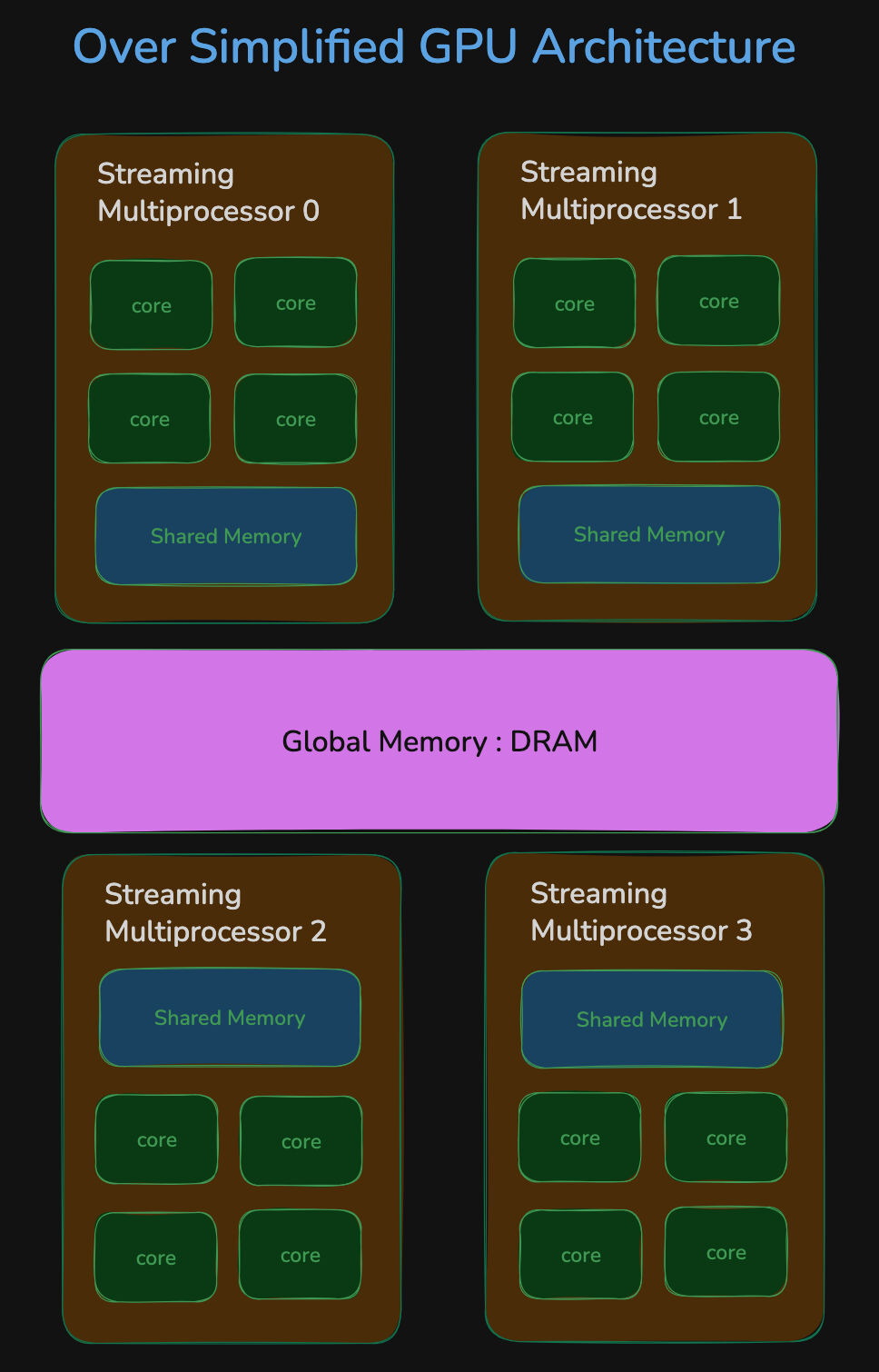
A Slight Detour Into GPU Architecture

So how does this map to GPUs? Just like the analogy above, GPUs also have tiered storage. There is large off-chip memory such as HBM or GDDR, which is what people usually mean when they talk about GPU memory. It is typically measured in tens of gigabytes. For example, an NVIDIA H100 has 80 GB of HBM. This is the analogue of the paper in our example.

On-chip storage is much smaller but physically much closer to the compute cores. In practice, what matters for kernels is registers plus shared memory and L1-like storage on each SM. That storage is far faster to access than HBM, but it is tiny by comparison, usually only tens to hundreds of kilobytes of directly useful scratchpad per SM rather than gigabytes. That is the closest match to the scratchpad in our analogy.

If you are careful about the implementation, you can avoid writing the full attention weights to DRAM and save a lot of time in the process.

One difference from the analogy is that a GPU has many compute units and many on-chip memories working in parallel, while they all still share the same DRAM.

The Math-e-Magics

The analogy is useful, but the key question is whether the math still works. It does. Each query row can be processed independently of the other query rows. The output for query $i$ depends on all keys and values, but it does not depend on the outputs of any other queries. That is similar to one row of long multiplication depending on one digit of the multiplier and all digits of the multiplicand.

\[s_{ij} = \frac{q_i \cdot k_j^T}{\sqrt{d}}, \qquad p_{ij} = \frac{e^{s_{ij}}}{\sum_{\ell=1}^{n} e^{s_{i\ell}}}, \qquad o_i = \sum_{j=1}^{n} p_{ij} v_j\]

So with that in mind, the tempting plan would be:

1. Load query $i$ into SRAM
2. Load key $j$ and value $j$ into SRAM
3. Compute $q_i \cdot k_j^T$ in SRAM
4. Perform the softmax operation
5. Compute $p_{ij} \cdot v_j$ in SRAM
6. Repeat steps 2-5 for all $j$
7. Maintain the running sum

The hurdle is softmax. That plan is not actually valid, because you need the whole row to compute softmax correctly. You cannot apply softmax element-wise and be done.

Life would be much easier without that dependency. That is one reason linear attention variants replace softmax with other mechanisms that let them fold the computation differently and avoid materializing expensive attention weights. Here, though, we still have softmax, so we have to handle it carefully.

The softmax problem

Given a row of values $x_1, x_2, \dots, x_n$, the softmax is

import numpy as np

def softmax(x):
    x_max = np.max(x)
    x_adjusted = x - x_max  # Subtract max for numerical stability.
    exp_x = np.exp(x_adjusted)
    output = exp_x / np.sum(exp_x)
    return output

For numerical stability, we subtract the row maximum before taking exponentials, especially when working in FP16. Consider

\[x = [10, 2, 1, 3, 5, 8, 16]\]

If you exponentiate $x$ directly, the largest term dominates and can overflow in formats like FP16:

\[e^x \approx [22026, 7.4, 2.7, 20.1, 148.4, 2981, \sim 9000000]\] \[x' = x - x_{\max} = [-6, -14, -15, -13, -11, -8, 0]\] \[e^{x'} \approx [0.0025, 0.000000091, 0.000000003, 0.000000335, 0.0000101, 0.000335, 1.0]\]

These values are much easier to represent without producing NaNs or infinities.

But this still introduces another dependency, because ideally you want the full row to know both the maximum and the denominator.

The key trick here is to compute a “partial softmax” and patch it up later.

So the plan is to

1. Keep the exponent stable as the row maximum changes
2. Calculate the denominator in a streaming fashion
3. Update the weighted value sum in a streaming fashion as well

Stabilizing the exponent

The key idea here is that we do not load just one key/value pair. We load a small block of those, say 64, compute a block of scores, and update a running summary for each query row. Let the full score row for query $i$ be $[s_{i1}, s_{i2}, \dots, s_{in}]$, partitioned into blocks $B_1, B_2, \dots, B_T$.

Before going to the full recurrence, let us see the smaller algebraic trick. Suppose we split a row into two chunks:

\[x = [x^{(1)}, x^{(2)}]\]

For each chunk, define

\[m^{(a)} = \max(x^{(a)}), \qquad \ell^{(a)} = \sum_j e^{x^{(a)}_j - m^{(a)}} \quad \text{(partial sum)}\]

and for the whole concatenated row define

\[m = \max(x) = \max(m^{(1)}, m^{(2)})\]

Then the denominator of the stable softmax can be rewritten as

\[\sum_j e^{x_j - m} = \sum_{j \in B_1} e^{x^{(1)}_j - m} + \sum_{j \in B_2} e^{x^{(2)}_j - m}\] \[= e^{m^{(1)} - m} \sum_{j \in B_1} e^{x^{(1)}_j - m^{(1)}} + e^{m^{(2)} - m} \sum_{j \in B_2} e^{x^{(2)}_j - m^{(2)}}\] \[= e^{m^{(1)} - m} \ell^{(1)} \quad \quad \quad \quad \text{(rescale old sum)} \\ + e^{m^{(2)} - m} \ell^{(2)} \quad \quad \quad \quad \text{(add new sum)}\]

That is the key identity. When the reference max changes, we rescale the old chunk to the new max and keep going.

The exact same trick works for the weighted numerator as well. If

\[u^{(a)} = \sum_j e^{x^{(a)}_j - m^{(a)}} v^{(a)}_j\]

then

\[u = \sum_j e^{x_j - m} v_j = e^{m^{(1)} - m} u^{(1)} + e^{m^{(2)} - m} u^{(2)}\]

Now we simply apply this same algebra repeatedly, one KV block at a time.

With initialization $m_i^{(0)} = -\infty$, $\ell_i^{(0)} = 0$, and $u_i^{(0)} = 0$, for the first $t$ blocks we maintain three quantities:

\[m_i^{(t)} = \max_{j \in B_1 \cup \dots \cup B_t} s_{ij}\] \[\ell_i^{(t)} = \sum_{j \in B_1 \cup \dots \cup B_t} e^{s_{ij} - m_i^{(t)}}\] \[u_i^{(t)} = \sum_{j \in B_1 \cup \dots \cup B_t} e^{s_{ij} - m_i^{(t)}} v_j\]

At the end, the output is simply

\[o_i = \frac{u_i^{(T)}}{\ell_i^{(T)}}\]

Now assume we are processing block $B_t$. Let

\[\tilde{m}_i^{(t)} = \max_{j \in B_t} s_{ij}, \qquad m_i^{(t)} = \max\left(m_i^{(t-1)}, \tilde{m}_i^{(t)}\right)\]

The old statistics were normalized with respect to $m_i^{(t-1)}$, but the new block must be merged using the newer and potentially larger max $m_i^{(t)}$. So we rescale the old accumulators before adding the new block:

\[\ell_i^{(t)} = e^{m_i^{(t-1)} - m_i^{(t)}} \ell_i^{(t-1)} + \sum_{j \in B_t} e^{s_{ij} - m_i^{(t)}}\] \[u_i^{(t)} = e^{m_i^{(t-1)} - m_i^{(t)}} u_i^{(t-1)} + \sum_{j \in B_t} e^{s_{ij} - m_i^{(t)}} v_j\]

This is the whole trick behind FlashAttention. We never materialize the full $n \times n$ attention matrix in DRAM. Instead, we keep a running max, a running denominator, and a running weighted sum for each query row, while processing one KV tile at a time on chip.

u_i = torch.zeros(n_q, d)          # running weighted value sum
l_i = torch.zeros(n_q, 1)          # running denominator
m_i = torch.full((n_q, 1), -torch.inf)

load_from_dram(q_i)                # q_i has shape [n_q, d]

for k_batch, v_batch in batched(zip(keys, values)):
    load_from_dram(k_batch)
    load_from_dram(v_batch)

    scores = torch.matmul(q_i, k_batch.transpose(-2, -1)) / math.sqrt(d)
    block_max = scores.max(dim=-1, keepdim=True).values
    new_max = torch.maximum(m_i, block_max)

    exp_scores = torch.exp(scores - new_max)
    old_scale = torch.exp(m_i - new_max)

    l_i = old_scale * l_i + exp_scores.sum(dim=-1, keepdim=True)
    # adjust old/running output and add current block's contribution
    u_i = old_scale * u_i + torch.matmul(exp_scores, v_batch)
    m_i = new_max  # update the running max

o_i = u_i / l_i
write_to_dram(o_i)  # the only thing we write back to DRAM

Triton Implementation

Triton implementation (click to expand)

Now let us map the exact same recurrence to Triton. The kernel below is intentionally kept educational:

• forward only
• one (sequence, head_dim) tensor per head
• non-causal attention
• comments only where the recurrence is not obvious

import math
import torch
import triton
import triton.language as tl


@triton.jit
def flash_fwd_kernel(
    q_ptr, k_ptr, v_ptr, o_ptr,
    stride_qm, stride_qk,
    stride_km, stride_kk,
    stride_vm, stride_vk,
    stride_om, stride_ok,
    N_CTX, D,
    sm_scale,
    BLOCK_M: tl.constexpr,
    BLOCK_N: tl.constexpr,
    BLOCK_D: tl.constexpr,
):
    pid_m = tl.program_id(0)

    offs_m = pid_m * BLOCK_M + tl.arange(0, BLOCK_M)
    offs_n = tl.arange(0, BLOCK_N)
    offs_d = tl.arange(0, BLOCK_D)

    # Load one tile of queries and keep it on SRAM for the whole KV sweep.
    q_ptrs = q_ptr + offs_m[:, None] * stride_qm + offs_d[None, :] * stride_qk
    q_mask = (offs_m[:, None] < N_CTX) & (offs_d[None, :] < D)
    q = tl.load(q_ptrs, mask=q_mask, other=0.0)

    # These are exactly the running statistics from the math above.
    # we chose to do these in float32 for higher precision and range.
    # This incurs some more additional cost but wouldn't effect the order of magnitude
    m_i = tl.full((BLOCK_M,), float("-inf"), dtype=tl.float32)
    l_i = tl.zeros((BLOCK_M,), dtype=tl.float32)
    acc = tl.zeros((BLOCK_M, BLOCK_D), dtype=tl.float32)

    # Iterate over batches of keys/values of size BLOCK_N
    for start_n in tl.range(0, N_CTX, BLOCK_N):
        k_ptrs = k_ptr + (start_n + offs_n)[:, None] * stride_km + offs_d[None, :] * stride_kk
        v_ptrs = v_ptr + (start_n + offs_n)[:, None] * stride_vm + offs_d[None, :] * stride_vk
        kv_mask = ((start_n + offs_n)[:, None] < N_CTX) & (offs_d[None, :] < D)

        k = tl.load(k_ptrs, mask=kv_mask, other=0.0)
        v = tl.load(v_ptrs, mask=kv_mask, other=0.0).to(tl.float32)

        # scores = q_i @ k_j^T / sqrt(d)
        qk = tl.dot(q, tl.trans(k)) * sm_scale

        # m_i^(t) = max(m_i^(t-1), block_max)
        block_max = tl.max(qk, axis=1)
        new_m_i = tl.maximum(m_i, block_max)

        # Rescale old state to the new max before adding the new block.
        p = tl.exp(qk - new_m_i[:, None])
        alpha = tl.exp(m_i - new_m_i)

        # l_i^(t) = exp(m_old - m_new) * l_i^(t-1) + sum(exp(scores - m_new))
        l_i = alpha * l_i + tl.sum(p, axis=1)

        # u_i^(t) = exp(m_old - m_new) * u_i^(t-1) + exp(scores - m_new) @ v
        acc = alpha[:, None] * acc + tl.dot(p, v)
        m_i = new_m_i

    # Final softmax and normalization
    out = acc / l_i[:, None]

    o_ptrs = o_ptr + offs_m[:, None] * stride_om + offs_d[None, :] * stride_ok
    o_mask = (offs_m[:, None] < N_CTX) & (offs_d[None, :] < D)
    # write O back to DRAM. The only DRAM write    
    tl.store(o_ptrs, out, mask=o_mask)


def flash_attn_triton(q, k, v):
    # q, k, v: [N_CTX, D] for a single head
    assert q.shape == k.shape == v.shape
    assert q.is_cuda and k.is_cuda and v.is_cuda

    N_CTX, D = q.shape
    o = torch.empty_like(q)

    BLOCK_M = 64
    BLOCK_N = 64
    BLOCK_D = triton.next_power_of_2(D)
    sm_scale = 1.0 / math.sqrt(D)

    grid = (triton.cdiv(N_CTX, BLOCK_M),)
    flash_fwd_kernel[grid](
        q, k, v, o,
        q.stride(0), q.stride(1),
        k.stride(0), k.stride(1),
        v.stride(0), v.stride(1),
        o.stride(0), o.stride(1),
        N_CTX, D,
        sm_scale,
        BLOCK_M=BLOCK_M,
        BLOCK_N=BLOCK_N,
        BLOCK_D=BLOCK_D,
        num_warps=4,
        num_stages=2,
    )
    return o

The mapping from math to code is direct:

• m_i stores the running row max
• l_i stores the running denominator
• acc stores the running weighted value sum
• alpha = exp(m_old - m_new) is the rescaling factor that lets us merge blocks safely

Production kernels go quite a bit further than this. They add causal masking, better work partitioning, descriptor-based loads, tuning for different head dimensions, and backward kernels. But the core idea is exactly the same as the recurrence we derived above.

Analysis

So the math checks out. The subtle but important point is that FlashAttention does not change the asymptotic amount of arithmetic in attention. You still have to look at every query-key pair, so the compute stays on the order of

\[\Theta(n^2 d)\]

The win comes from data movement and peak memory, not from magically removing the quadratic interaction itself.

Let $B$ be the DRAM-SRAM bandwidth and $C$ be the compute throughput. We will use a simplified BF16 accounting where each element takes 2 bytes.

Standard attention

Under the usual two-stage implementation, we first compute $S = QK^T$ and store it, then we read $S$ back to compute $\text{softmax}(S)V$.

Step 1: Compute $S = QK^T$

• Read $Q$ and $K$: $\quad 2 \cdot (n d) \cdot 2 = 4nd$ bytes
• FLOPs for $QK^T$: $\quad 2n^2d$
• Write $S \in \mathbb{R}^{n \times n}$: $\quad 2n^2$ bytes

Step 2: Compute $O = \text{softmax}(S)V$

• Read $S$ and $V$: $\quad 2n^2 + 2nd$ bytes
• FLOPs for $PV$: $\quad 2n^2d$
• Softmax itself is element-wise/reduction work on $n^2$ entries, so it adds $\Theta(n^2)$ operations
• Write $O \in \mathbb{R}^{n \times d}$: $\quad 2nd$ bytes

So in this simplified model, total DRAM traffic is

\[\underbrace{4nd}_{Q,K\ \text{read}} + \underbrace{2n^2}_{S\ \text{write}} + \underbrace{(2n^2 + 2nd)}_{S,V\ \text{read}} + \underbrace{2nd}_{O\ \text{write}} = 8nd + 4n^2 \text{ bytes}\]

and total compute is

\[2n^2d + 2n^2d + \Theta(n^2) = 4n^2d + \Theta(n^2)\]

If we convert that into a back-of-the-envelope time model, we get

\[T_{\text{standard}} \approx \frac{8nd + 4n^2}{B} + \frac{4n^2d + \Theta(n^2)}{C}\]

For long contexts, the painful term on the IO side is the $4n^2$ coming from writing and re-reading the attention matrix.

FlashAttention

Now let us do the same accounting for tiled attention. Let the query tile size be $b_q$ and the KV tile size be $b_k$. There are

\[\frac{n}{b_q} \quad \text{query tiles and} \quad \frac{n}{b_k} \quad \text{KV tiles.}\]

For one pair of tiles, the work is

Per tile compute

• $Q_i K_j^T$: $ \quad 2 b_q b_k d$ FLOPs
• Online softmax stats on the $[b_q, b_k]$ score tile: $\quad \Theta(b_q b_k)$ ops
• Multiply by values: $ \quad 2 b_q b_k d$ FLOPs
• Rescale and update the running output/statistics: $\quad \Theta(b_q d)$ ops

So one tile costs

\[4 b_q b_k d + \Theta(b_q b_k + b_q d)\]

Since there are $\frac{n}{b_q} \cdot \frac{n}{b_k}$ such tiles, the full compute becomes

\[\frac{n}{b_q} \cdot \frac{n}{b_k} \left(4 b_q b_k d + \Theta(b_q b_k + b_q d)\right)\] \[= 4n^2 d + \Theta\left(n^2 + \frac{n^2 d}{b_k}\right)\]

So again, the arithmetic is still quadratic in sequence length.

For IO, assume the current query tile and its running accumulators stay on-chip while we sweep over all KV tiles. Then for one query tile:

• Read $Q_i$: $\quad 2 b_q d$ bytes
• For each KV tile, read $K_j$ and $V_j$: $\frac{n}{b_k} \cdot 4 b_k d = 4nd$ bytes
• Write final $O_i$: $\quad 2 b_q d$ bytes

So one query tile costs

\[2 b_q d + 4nd + 2 b_q d = 4 b_q d + 4nd\]

Across all $\frac{n}{b_q}$ query tiles, total DRAM traffic is

\[\frac{n}{b_q}(4 b_q d + 4nd) = 4nd + \frac{4n^2 d}{b_q}\]

up to lower-order bookkeeping terms for $m_i$ and $\ell_i$.

This is the detailed reason FlashAttention helps. We replace the explicit $n \times n$ score-matrix traffic with repeated reads of much smaller $K,V$ tiles. The exact crossover depends on the head dimension, tile sizes, occupancy, and memory system, but the key point is that IO now scales with tiles rather than with materializing and re-reading a full score matrix.

That is where the wall-clock win comes from.

So the rough time model becomes

\[T_{\text{flash}} \approx \frac{4nd + \frac{4n^2 d}{b_q}}{B} + \frac{4n^2d + \Theta\left(n^2 + \frac{n^2 d}{b_k}\right)}{C}\]

The important bit is not that the quadratic interaction disappears. It does not. The important bit is that the quadratic DRAM-sized attention matrix disappears.

Another way to say the same thing is:

• Standard attention: arithmetic $\Theta(n^2 d)$, intermediate memory $\Theta(n^2)$
• FlashAttention: arithmetic $\Theta(n^2 d)$, no extra $\Theta(n^2)$ attention matrix in DRAM, plus a tile-sized on-chip working set

In FlashAttention, the on-chip working set for one query tile is roughly

\[Q_i \in \mathbb{R}^{b_q \times d}, \quad K_j \in \mathbb{R}^{b_k \times d}, \quad V_j \in \mathbb{R}^{b_k \times d}, \quad u_i \in \mathbb{R}^{b_q \times d}, \quad \ell_i, m_i \in \mathbb{R}^{b_q}\]

plus transient score or probability fragments of size about $b_q \times b_k$, depending on how the kernel schedules the computation. So the on-chip footprint is, instead of needing space for an $n \times n$ matrix, on the order of

\[\Theta\big((b_q + b_k)d + b_q b_k\big)\]

Results

Let’s take a quick look at the performance and memory usage of the two implementations.

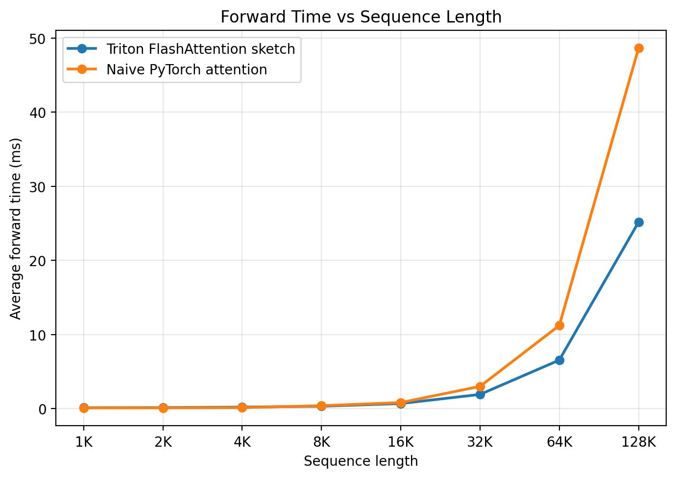
The companion benchmark script measures forward-pass BF16 attention and reports the peak memory used by the attention operation. In the run shown here, the Triton kernel is still an educational sketch rather than a production-quality kernel, so the speedup on the B200 is modest. With auto-tuning, better partitioning, and a more optimized implementation, you should expect better numbers.

As for memory, FlashAttention uses far less than standard attention, as shown below:

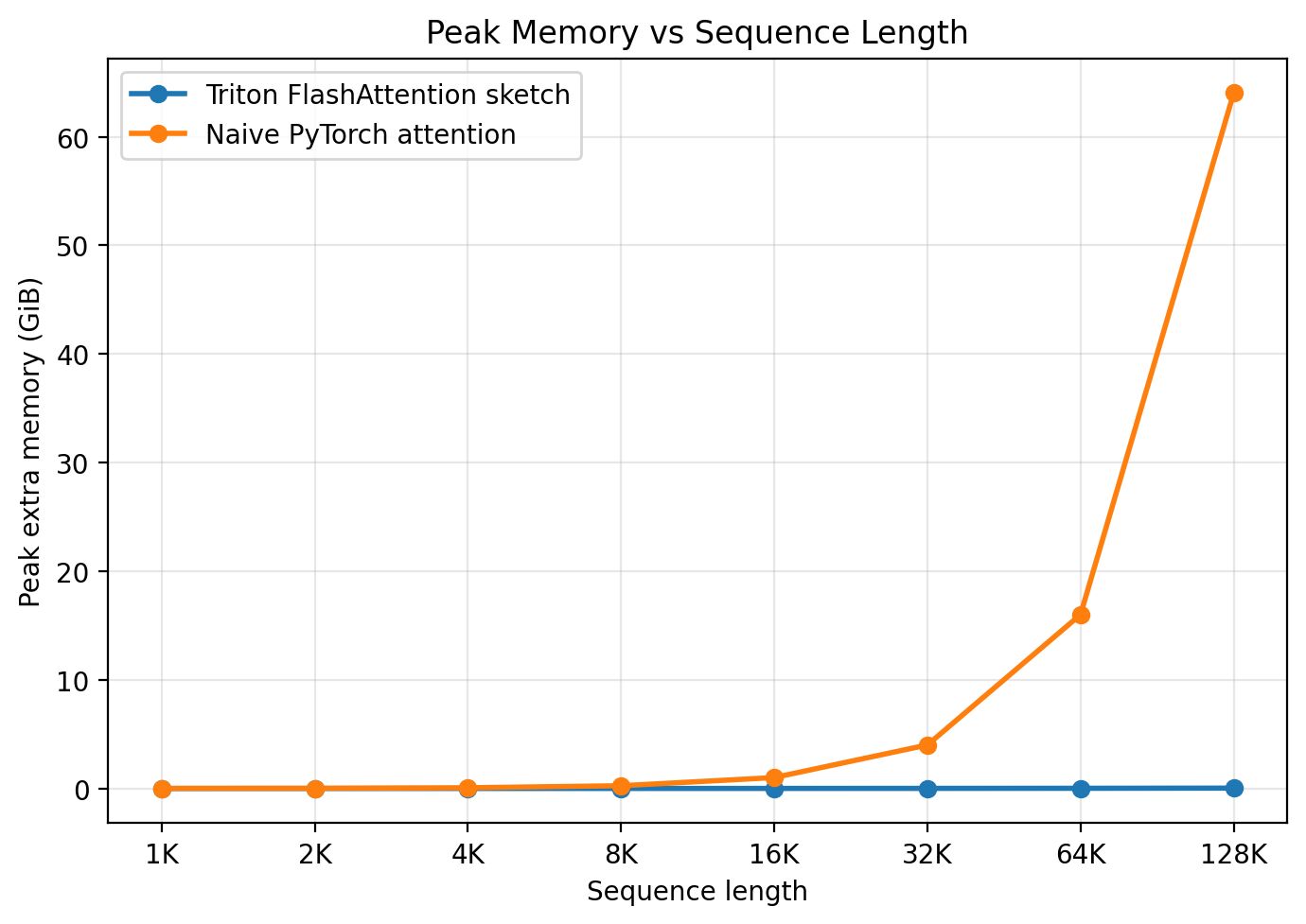
It almost looks as if the memory usage does not increase with sequence length. That is not a bug, but it is easy to misread. FlashAttention still has memory use that grows with sequence length because the inputs and outputs still grow. What disappears is the extra quadratic-sized score tensor. On a linear-scale plot, the quadratic growth of the baseline drives the axis so high that the much smaller increase from FlashAttention becomes hard to see. The log plot below makes the difference in slopes much clearer.

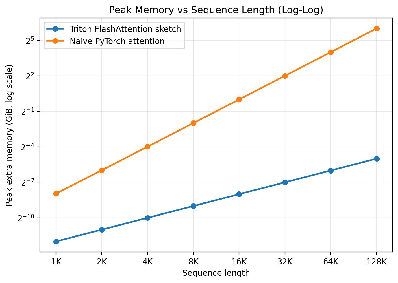
Notice the difference in slope between the two lines there. It is a useful exercise to reason through why the slopes differ and by how much analytically.

A Few More Things and Final Thoughts

One thing I intentionally skipped here is the backward pass. In many training setups, people use gradient checkpointing, which means activations are either offloaded or discarded and recomputed during backpropagation. FlashAttention uses the same general idea there as well: save a small amount of summary state, then recompute what you need instead of storing the full attention matrix. Many of the same gains show up in the backward pass too, sometimes even more strongly. I may cover the backward pass of FlashAttention in a future post, but this one is already long enough.

This is a good example of how much performance you can recover just by thinking carefully about systems and data movement. I have written previously about how tensor parallelism approaches can be combined to reduce inter-GPU communication during inference in systems like vLLM. FlashAttention is another case where the real win comes from how the computation is scheduled and stored, not from changing the high-level objective.

That is it from my side for today. Feel free to share your thoughts, comments and feedback. Will be back again with more mathematricks! Until then, Ciao!

References

• FlashAttention paper
• FlashAttention repo
• Online softmax implementation