The lore behind LoRA

Introduction

Previously we have talked about Transformer and attention being re-imagined from the first principles. We’ve motivated the need for attention, MLP, MoE and how they work in theory. But so far we’ve only talked about how these work in theory. But for the said components to work in ideal way, we need to train the model. Today we try to understand how to efficiently (we will explain this in a while) do that.

A brief about standard training

So when training LLMs, assuming that we have data of seq_len tokens, each data sample gives us seq_len-1 training examples all in one, namely, the subsequence of tokens starting from position 0 to i for all i from 0 to seq_len-2 as the input and the token at position i+1 as the target. All this is done in a single pass through the language model. Once a token is predicted, we calculate the Cross Entropy Loss and backpropagate the gradients through the entire model. I’m intentionally cutting the explanation short here about the training process and the reason behind all these. If you are interested, I might write another going into few more details about standard LLM training. But for now, lets move on to the main topic.

Everything that touches the GPU

When training LLMs, one of the biggest constraints we have is GPU memory. People come up with clever ways like parallelisms to circumvent this problem but it exists nonetheless. Let us see what all components are involved when training models.

• Model weights/Parameters: We store the weights in memory to perform forward and backward passes. For simplicity assume that each parameter is a BF16/FP16 number which takes up 2 bytes of memory. For a model with N parameters, we need 2N bytes of memory.
• Activations: When doing computations, there are intermediate results that sit on our GPU. For example, the output of layer 1 in a multi layer transformer is an activation. So is the output of the last layer. The size of this depends primarily on the input size and model configuration. Larger the input, larger the activations.
• Gradients: This is how we train/improve the model. We calculate gradients of the loss wrt each of the parameter and use them to update the parameters. This is what contributes to gradient descent. Each trainable parameter contributes to one gradient.
• Optimizer states: Once you calculate the said gradients, you need to have a mechanism to update the parameters using the said gradients. Sometimes you wanna normalise the gradients, sometimes you want to keep a moving average of the gradients. This is where optimizer and optimizer states come in. optimizer dictates the math while optimizer states are the values you use to perform the math. For simple SGD, we have $w_{t} = w_{t-1} - lr * g_{t}$ where $g_{t}$ is the gradient at time $t$ and $lr$ is the learning rate. For Adam, we have $m_{t} = beta_1 * m_{t-1} + (1 - beta_1) * g_{t}$ and $v_{t} = beta_2 * v_{t-1} + (1 - beta_2) * g_{t}^2$ where $m_{t}$ and $v_{t}$ are the moving averages of the gradients and their squares respectively. Then we have $w_{t} = w_{t-1} - lr * m_{t} / (sqrt(v_{t}) + epsilon)$ where $epsilon$ is a small constant to prevent division by zero. So each trainable parameter needs a few optimizer states.

So what?

Well you see where we’re going with this. For typical AdamW optimizer based training, for an N parameter model, we’d end up needing at least 2N * 4 bytes of memory just for the parameters, gradients and optimizer states. Note that typically you store these things in higher precision but we’re just assuming a simplistic scenario here for convenience.

For a 7B parameter model, you’re looking at 14GB of weights, 14GB gradients and 28GB of optimizer states. That’s 56GB of memory just for the parameters, gradients and optimizer states! Note that we assumed BF16 everything, in practice people use FP32 and that blows it up even more.

Generally with LLMs, they are trained on trillions of tokens of data. For example, llama 3 has been trained on 15T tokens and Qwen3 family has been trained on 36T tokens. When you are fine tuning to a specific use case, you generally train on the order of millions of tokens (not even billions). So you are essentially training on a tiny tiny fraction of the data that the original model was trained on. The model has already learnt language, grammar, code, math, science etc. You are just exposing it to a new flavor. At that point, do you really need to train every single parameter?

How does it matter

Well you see, if we keep the model the same, the model parameter and activations do not change by much. What changes is the gradients and optimizer states because they hinge onto the trainable parameters rather than the total parameters. So if we can somehow reduce the number of trainable parameters, even while increasing total parameters, we’re still at a win especially when using optimizers like Adam.

Mathematically speaking, memory usage can be written as:

\[\begin{align*} \text{Memory} &= \text{Model Params} + \text{Activations} + \text{Gradients} + \text{Optimizer States} \\ &\sim 2N_{total} + j \times N_{trainable} + k \times 2N_{trainable} \\ \text{where } j \text{ and } k & \text{ are constants for dtype and number of states} \end{align*}\]

There are many ways you can go about doing this. Typically what people used to do in the days of CNN for image recognition was to use ResNet and freeze (not train) almost all of the initial layers and just update the last layer. So a model that has already learnt to recognise edges, corners, shapes etc. can be used as a base and we just need to update the last layer to recognise our specific task for example, from classifying between 100 classes to classifying between cats 🐈 and dogs 🐕.

The same can be applied to LLMs. We can freeze majority of the model while training LMHead and maybe a layer or two here and there. In theory this works. But ask yourself a couple of questions here. In transformers, if each layer is identifying some unique patterns and sometimes work independently, how do you know that your task can be represented by just updating only the last layer (or any subset of layers for that matter)?

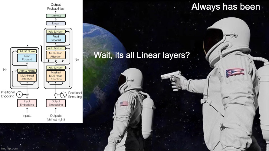
So ideally, we need to figure out a way to update every layer. But in transformer layer themselves, there are multiple components like query, key, value, output projection, MLP etc. How do we know which components to update and which to freeze? Well, what is the underlying architecture for all the said components? Yeah, everything is a linear layer. So if we can find a way to train a linear layer in a parameter efficient way, we can apply it to all the components, all layers and almost* all models.

Linear Layers everywhere

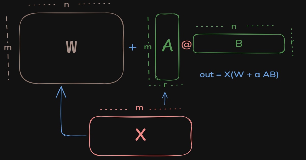
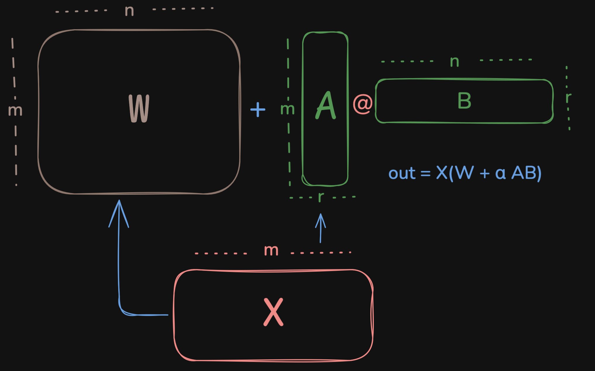
So one of the most basic and most prevalant computations through out the transformers is the linear layer which does out = X@W where X is the input, $W \in \mathbb{R}^{m \times n}$ is the weight matrix. Upon updating, we’d have out = X@(W + delta_W) where delta_W is the change in the weight matrix. If we can somehow find a way to represent delta_W using fewer parameters, we can achieve parameter efficient training. But we are also constrained by the fact that the shape of delta_W must match the shape of W which is (m,n).

All linear layers in a transformer

One good property of matrices we can exploit is that if you multiply two matrices, the inner reduction dimension vanishes. So if you multiply matrices of shapes (m,r) with (r,n), the r goes off and you’ll be left with a matrix of shape (m,n). While doing so, if the resultant decomposition can have lesser number of parameters than the original/output matrix. Let us mathematically see when that happens.

We ideally need m*r + r*n « m*n for this to make sense. So r << m*n/(m+n). At that scales assuming m~n, we’d need r << n/2. If you look at the example of Qwen 3 0.6B, the hidden size is 1024 and intermediate size is 3072. So our m, n are at least 1024 here. But this only gave us an upper bound on the inner size of the decomposed matrices.

If you are familiar with the concept of a rank, then you’d know that rank(AB) <= min(rank(A), rank(B)). And also $rank(X \in \mathbb{R^{x,y}}) \leq \min(x,y)$. So for the $W_{delta}$ we talked about, we have $rank(W_{delta}) \leq \min(rank(A), rank(B)) \leq \min(\min(m,r), \min(r, n)) = r $. So we are imposing a Low Rank structure on the weight update matrix. If you want the model to learn complex patterns, this kind of puts a restriction on the capability of the model. So we do not want r to be too low that it hinders learning. Typically you see it taking values like 8, 16, 32 for simpler tasks and sometimes higher for complex tasks (which is very rarely the case).

At typical scales as we discussed, r = 16 and m,n~1024, we added $A \in \mathbb{R}^{m \times r}$ and $B \in \mathbb{R}^{r \times n}$ parameters for every $W \in \mathbb{R}^{m \times n}$ matrix. So we added $16 * (1024 + 1024) = 32768$ parameters for every $1024 \times 1024$ matrix, which is just 3% of the original parameters. For bigger models or for lower ranks this is even lower. This is why we call it efficient. We only need to track the gradients and optimizer states for these 3% parameters. These are the main characters of the story. Rest all are just helpers :)

So for training a 7B model, we’d still need the 14GB of weights. We also added say 3% aka 200M parameters for the adapters. This amounts to 200MB of more space for parameters. But we only need the gradients and optimizer states for the said 200M parmaeters which comes out to around 600M parameters or 1.2GB memory. Overall, if the activations are small enough (with gradient checkpointing), we’re looking at around 15-16GB of memory for training a 7B model with LoRA adapters! This is huge savings compared to the 56GB we were looking at previously. This is what made finetuning accessible to the GPU poor like us.

Formalising

For every linear layer with weight $W \in \mathbb{R}^{m \times n}$, we decompose it as $W = W_0 + \Delta W$ where $W_0$ is the original weight and $\Delta W$ is the update. We can write $\Delta W = \alpha \cdot A \times B$ where $A \in \mathbb{R}^{m \times r}$ and $B \in \mathbb{R}^{r \times n}$ and $\alpha$ is a fixed scalar. We set A and B as trainable and keep $W_0$ frozen. The $\alpha$ is to keep the contribution of LoRA in check and consistent across ranks. We do not want high rank to influence the output in terms of magnitude.

In practice, these are called adapters.

LoRA visualised

Now we need to define how the matrices are initialised right? Right initialisation can go a long way. I have previously experimented with different initialisation strategies. But for now, lets stick to the basics.

What do we want from LoRA? At the worst, it should not disturb the base model. So we want the initialisation to be such that it doesn’t affect the compute to begin with (until it is trained).

So we want $(W + \Delta W_{init}) \cdot X = W \cdot X$ aka $A_{init} \cdot B_{init} \cdot X = 0^{m \times n}$. This should happen irrespective of what the input $X$ is. So the only way to make this is happen is to initialisae to that $A_{init} \cdot B_{init} = 0^{m \times n}$. In practice, as you see below, one of the matrices (generally B) is initialised to all zeros while the other can pick any initialisation. This might be tingling your spidey senses that all zeros is advised against in deep learning in general. But here the presence of $W$ avoids the said issue. People have tried alternative initialisations to avoid all zero init. But this is still the standard.

Implementation

If you speak in code, here’s the extract from the peft:

# creating matrices/linear layers of (m,r) and (r,n) shapes
self.lora_A[adapter_name] = nn.Linear(self.in_features, r, bias=False)
self.lora_B[adapter_name] = nn.Linear(r, self.out_features, bias=lora_bias)
# How these are initialised
nn.init.kaiming_uniform_(self.lora_A[adapter_name].weight, a=math.sqrt(5))
nn.init.zeros_(self.lora_B[adapter_name].weight)

and here’s how they are used for computation

# base_layer is the original linear layer with weight `W`
result = self.base_layer(x,)
# Notice here we do B@A because we do X@W in pytorch and not W@X :)
result = result + lora_B(lora_A(dropout(x))) * scaling

If you use unsloth, you just do

from unsloth import FastLanguageModel

model = FastLanguageModel.get_peft_model(
    model,
    r=16, # dictates the rank of the decomposition. higher is better but causes slightly more memory usage
    # Which linear layers is the lora supposed to be applied to 
    target_modules=["q_proj", "k_proj", "v_proj", "o_proj", "up_proj", "down_proj", "gate_proj"],
    lora_alpha=32, # defines the multiplier
)

If you use peft, it automatically converts your Linear layers into LoRA layers. Typically for a model, you can do this by doing

from peft import get_peft_model, LoraConfig
peft_config = LoraConfig(
    r=16,
    lora_alpha=32,
    target_modules=["q_proj", "k_proj", "v_proj", "o_proj", "up_proj", "down_proj", "gate_proj"],
)
model = get_peft_model(model, peft_config)

The two ways to go about it

If you multiply two matrices of shapes (m,k) and (k,n), you’d be doing roughly 2mnk operations. To imagine, for every element in the output of shape (m,n) you’d be doing a sum of k multiplications aka $C[i,j] = \sum_{l=1}^{k} A[i,l] \cdot B[l,j]$.

There are two ways to compute the LoRA contribution because matrix multiplication distributes over addition, i.e. $X(W + AB) = XW + XAB$.

Method 1, the merged LoRA:

1. $W_{delta} = A \cdot B$
   • (m,r) @ (r,n) → (m,n): 2mnr operations
   • stores a weight of shape (m,n)
2. $W_{final} = W + W_{delta}$
   • (m,n) + (m,n) → (m,n): mn operations
   • can be done in-place if allowed, otherwise may need another buffer of shape (m,n)
3. $result = X @ W_{final}$ where X is the input of shape (s,m)
   • (s,m) @ (m,n) → (s,n): 2smn operations
   • output of shape (s,n)

Total operations: $2mnr + mn + 2smn$
Extra temporary memory: roughly $mn$ elements, dominated by storing $W_{delta}$

Method 2, the split LoRA:

1. $result_1 = X @ W$
   • (s,m) @ (m,n) → (s,n): 2smn operations
   • output of shape (s,n)
2. $tmp = X @ A$
   • (s,m) @ (m,r) → (s,r): 2smr operations
   • output of shape (s,r)
3. $result_2 = tmp @ B$
   • (s,r) @ (r,n) → (s,n): 2srn operations
   • output of shape (s,n)
4. $result = result_1 + result_2 * scaling$
   • (s,n) + (s,n) → (s,n): sn operations

Total operations: $2smn + 2smr + 2srn + sn$
Extra temporary memory: roughly $sr$ elements, dominated by storing $tmp = X @ A$

We’ll now see when split LoRA is more efficient in terms of compute.

We want $2smn + 2smr + 2srn + sn \le 2mnr + mn + 2smn$.

Cancelling $2smn$ from both sides gives $2smr + 2srn + sn \le 2mnr + mn$.

Factoring out $s$ on the left gives $s(2mr + 2rn + n) \le 2mnr + mn$.

So we get $s \le \frac{2mnr + mn}{2mr + 2rn + n} = \frac{mn(2r + 1)}{2r(m+n) + n}$.

If we additionally assume $m = n$, this becomes $\boxed{s \le \frac{m(2r+1)}{4r+1} \sim \frac{m}{2}}$ for moderate or large $r$.

In terms of memory usage, split LoRA is cheaper when the temporary tensor it materialises is smaller than the temporary tensor materialised by merged LoRA.

That is, we want $sr \le mn$.

So split LoRA is more memory efficient when $s \le \frac{mn}{r}$.

If we additionally assume $m = n$, this becomes $\boxed{s \le \frac{m^2}{r}}$.

Since in practice $r \ll m,n$, this memory condition is usually much easier to satisfy than the compute condition.

In reality there are other factors that dictate the time taken but this is just a theoritical analysis. Most GPU operations are memory bound. So the less memory you need to transfer, the faster your operations go.

So at training time, you benefit a lot from split LoRA. But at inference time, if you are sure of only serving the updated model, you are better of merging the weights and creating a final model and serving it. This reduces the compute done in inference path and can speed up inference by up to 30% on vLLM. Source: Trust me bro :)

We have done the same analysis has been done and the said changes have been implemented for MoE in Unsloth.

When you compare it to a simple linear layer, you are essentially adding more compute on top of the linear layer. Given that we reduce the memory usage for training by a lot and also the fact that gradients update and optimizer state update need not be done for all the parameters, we essentially end up saving some compute as well compared to the full fine-tuning.

LoRA in practice

LoRA is orthogonal to how you modify the base layer weights. So quantizing the base weights and adding LoRA on top of them has become a common theme when it comes to supervised fine tuning. This is typically referred to as QLoRA when you quantize the weights to 4bit. So the gradients and optimizer states still stay in relatively high precision while the base computation happens in lower precision, thus saving quite a lot of memory.

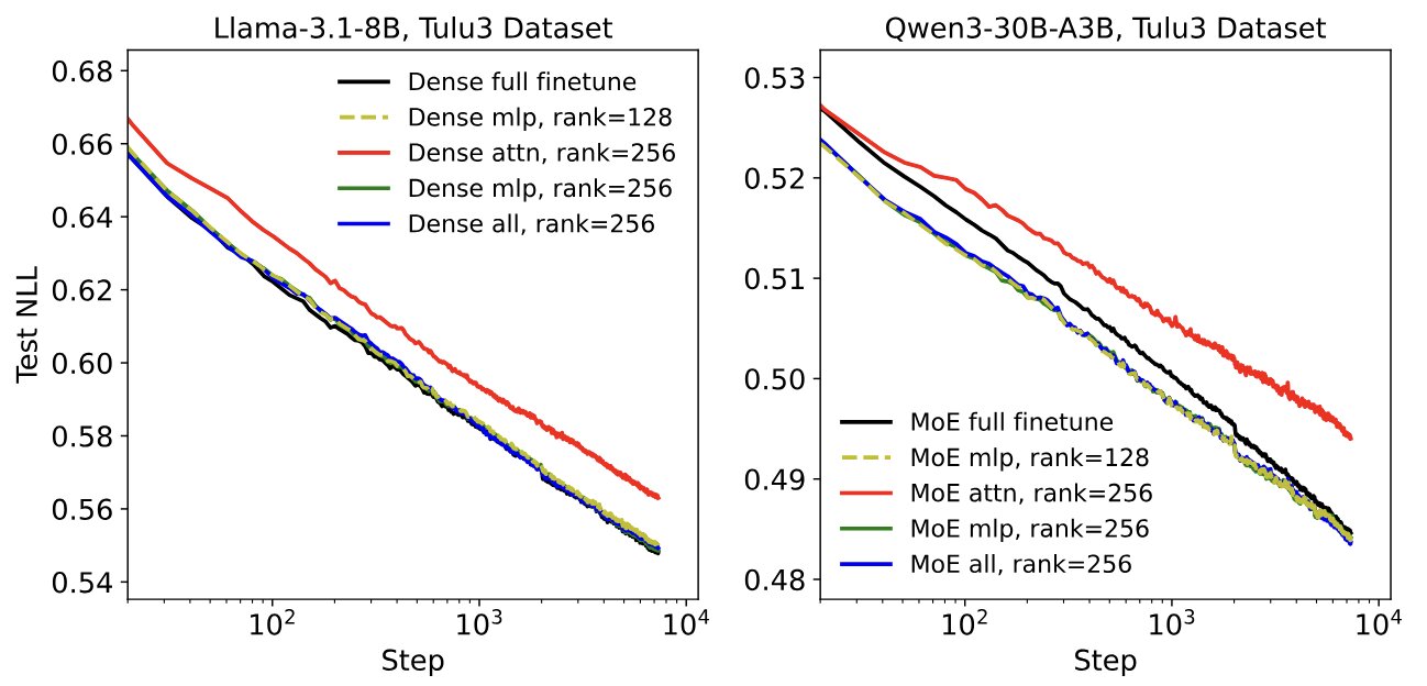
When doing reinforcement learning with LLMs people traditionally operate within the trust region to avoid the model drifting off too far from the original baseline. LoRA, in a way, acts as a good regularizer to make sure that the drift is not too much. Thinking Machines Lab has performed extensive experiments with LoRA for reinforcement learning and found out that it can be as good as training the entire model. Similar observations have been made for supervised fine-tuning as well.

LoRA thinky

What more does that give us

Well GPU memory savings is something we already established. That is why we formulated all this. But does it give us any more flexibility? The answer is an astounding yes. Given that it takes very little memory on GPU, in decomposed form, the same can be stored directly to disk and be loaded on demand. This means multiple things

• Sharing adapters is easy. You do not need to store/share gigabytes of full model weights
• Enabling or disabling adapter is easy. You just skip the $W_{delta}$ computation and you get the original model back :)
• You can serve multiple adapters at once and choose dynamically based on the task.
• Infact you can stack multiple adapters and use them together for a given task too.
• You can customise which layers, which modules you want to apply lora to. In theory you can pick say every 4th layer and apply lora to only k_proj there and that would work too, albeit not as good as adding it on everything

Final thoughts

This is just an introductory write-up on LoRA and how to go about thinking about LoRA. You can come up with many modifications, like orthogonal initialization or splitting decomposition in terms of magnitude and direction, like Dora does. The space for exploration is quite vast and also the compute requirement for doing the same is quite low so which is quite appealing. I’d strongly recommend you to try to think of alternatives that one can come up with and see how they perform. At the very least, read my previous blog on trying out different initialization schemes for LoRA here.

References

1. LoRA, DoRA, QLoRA
2. LoRA without regret