Attention and Transformer Imagined

Attention and Transformer Imagined

Introduction

Understanding language is an essential part to understanding knowledge. The meaning of understanding might vary depending on your setting. But the key idea is to somehow internalise the notion of language and be able to respond or act in certain ways. One way people try to internalise language is by trying to predict a word given a sequence of words. The idea is, if you can consistently correctly predict the next word, you’d have understood the given sequence of words, how all the words in the language interact with each other and what constitutes to a meaningful action/response.

Language has a lot of patterns. Grammar is a way of defining those patterns. So, the simplest way to model language is to statistically predict the most common continuation. Mathematically speaking it is a conditional probability distribution.

\[w^* : \arg \max_{w} P(w_{t+1} | w_1, w_2, \ldots, w_t)\]

where $w_{t+1}$ is the next word, $w_1, w_2, \ldots, w_t$ is the sequence of words.

This is a very simple model. It just is a static map from the sequence of words to its frequency. It doesn’t take into account the context of the words. It doesn’t take into account the grammar of the language. It doesn’t take into account the semantics of the words.

But this approach has a problem. To estimate the probability of the next word accurately, you might need to look at a long history of previous words (a long context). If you use traditional methods, like the one your smartphone keyboard probably uses, where you count frequencies of all possible sequences of n words, the number of possible sequences explodes exponentially with n. It quickly becomes impossible to store and learn from such sparse data.

The word vectors

What is a better way to model language? Now if you assume that each word is represented by numbers, you can do some funny math. But is one number enough to represent a word? The amount of information that a single word encompasses cannot be compressed into a single number. So you ideally need a set of numbers to represent a word. We generally call this a vector. So each word is represented by a vector.

\[w = [w_1, w_2, \ldots, w_n]\]

where $w_i$ is the $i$-th number in the vector.

Given that you have a set of vectors, one representing each word, what is the simplest way to predict the next word? We can simply add up all the vectors and find the word that is the most similar to the sum. The problem with this approach is, the sum might be arbitrarily large. Why is that a problem?

Imagine two sentences with almost same words. But one sentence is a repeat of the other one. You would want to predict the same word for both the sentences. But if you take the sum of those word vectors, in the case of larger sentence, the result would be very different from the case of smaller sentence.

For example, if you have the following sentences:

• What is the capital of India?
• What is the capital city of India?
• What city is the capital city of India?

The answer to all these questions is still the same. But having more occurances of the word “capital” would push the answer much more towards the word “capital”, hence away from the original answer “Delhi”.

How do we then tackle these two issues? One approach that comes to mind is average. Average is a very good operation to consider. Much better than just a summation. This solves the problem of the sum being arbitrarily large.

\[w = \frac{1}{n} \sum_{i=1}^n w_i\]

where $w_i$ is the $i$-th word vector.

But unfortunately, there is a big problem with averaging. Not all words are equally important for predicting the next word. So you would want to incorporate some notion of importance. We can do this by assigning a weight to each word.

\[w = \frac{\sum_{i=1}^n c_i w_i}{\sum_{i=1}^n c_i}\]

where $w_i$ is the $i$-th word vector weighted by a constant $c_i$. Note that $c_i$ is a independent of the input. This poses another problem. Even though the sentences are similar to the most part, the next token might be very different. For example, if you have the following sentences:

• Australia and South Africa played the World Test Championship Final 2025. South Africa defeated Australia. The winner is….
• Australia and South Africa played the World Test Championship Final 2025. Australia defeated South Africa. The winner is….

We’d still assign the same weight to the word “Australia” and “South Africa” even though the next token is very different. So we need a way to assign the weights depending on what we have seen so far.

Attention

The idea of attention is to assign a weight to each word based on what we have seen so far. This is a very powerful idea. It allows us to capture the context of the words.

\[w = \sum_{i=1}^n f(w_{1:n}, i) w_i\]

where $w_i$ is the $i$-th word vector weighted by a function of the input sequence. $w_{1:n}$ represents $[w_1, w_2, \ldots, w_n]$. $i$ is the index of the word in the sequence. Note that once such weights are computed, we can normalise them later to make sure we are not going out of range.

This shifts our focus to finding the function $f(w_{1:n}, i)$ that can help us predict the next word. We need a few key properties for this function.

1. It should be a function of the input sequence.
2. It should not depend on the length of the input sequence.
3. It should return a single real number representing some importance.

One such function is the similarity between the words in contention. Note that the similarity can be of some arbitrary transformation of the word vectors.

The formulation

So we can define the function as:

\[f(w_{1:n}, i) = \text{similarity}(w_i, w_n) \text{ or } \text{similarity} (\text{transformation}_1{(w_i)}, \text{transformation}_2{(w_n)})\]

You must be wondering why do we need to transform the vector before capturing similarity. There’s a neat reason for doing so. This way you can have different transformations of the same vector that lead to different relationships.

Consider the word bat. It can mean one of the following:

• (n) A flying animal
• (n) A cricket bat
• (n) A baseball bat
• (v) The act of batting

To determine whether the occurance is one of the above, you can ask different questions. Whether it is in the context of an animal or living being or whether it is in the context of a sport. Even then both might co-occur in the same sentence. So to take cure of multiple such words carrying multiple differnt meanings based on the context, you might want to capture multiple relationships/similarities for/with the same word.

So the usage of transformation to capture multiple relationships/similarities for/with the same word is justified.

Now you may wonder why do we need two different transformations $\text{transformation}_1$ and $\text{transformation}_2$. Why not just one?

The reason is the difference between what the word has to offer vs what the word wants to enquire from other words. It might want to show one form for fetching information and another form for providing information. This also leads to a very interesting advantage. You can capture multiple relationships by altering either one or both of the transformations. So like, $tr_{1,q}(w_i) \text{ and } tr_{2,k}(w_n) \text{ for } q \in Q, k \in K$ will capture $|Q| \times |K|$ different relationships.

The similarity

How do you now capture similarity between two vectors? The simplest way is to take the dot product. You might also be thinking of using cosine similarity. But both capture the same thing (upto certain scaling factors depending on the lengths of the vectors). The advantage of using dot product is that it is computationally efficient, especially on modern hardware (GPUs/TPUs) which are optimized for matrix multiplications.

\[\text{similarity}(w_i, w_n) = w_i \cdot w_n^T \in \mathbb{R}\]

The transformations

We need to define the transformations. The simplest transformation is a linear transformation. This can be done by multiplying with a matrix of appropriate dimensions. This is powerful because a linear transformation is a combination of rotation, scaling, and projection. And of course, the hardware now a days is very much optimised for such operations.

For a vector $w$ and a matrix $M$, the transformation can be defined as $wM$. This poses a restriction on the shape of the matrix. If $w \in \mathbb{R}^d$, then $M \in \mathbb{R}^{d \times h}$ for some $h$. We still have the flexibilty to choose $h$ as we want. The output is an $h$ dimensional vector.

The task of capturing similarity poses another restriction. The two transformations should end up in the same dimensional space. So if we define our Key transformation as $w@M_k$ and our Query transformation as $w@M_q$, we have $M_k \in \mathbb{R}^{d \times h}$ and $M_q \in \mathbb{R}^{d \times h}$ for some $h$.

Along with this, we also transform the vector to get the Value vector. This transformation gives meaning to the weighted average. Instead of passing the raw word vector $w_i$, we pass a transformed version, $w_i@M_v$. This allows the model to learn what information from that word is most useful to pass on.

So instead of $\sum c_i w_i$ we can have $\sum c_i (w_i@M_v)$ where $M_v \in \mathbb{R}^{d \times h_v}$. Note that the dimension of the value vector, $h_v$, can be different from $h$.

In general, if we have $n_h$ sets of (Query, Key, Value) transformations, we can have $n_h$ different “attention heads”. Each head can focus on a different type of relationship. We thus concatenate all the parts to get the final output vector.

Note: Technically speaking, we can leave the vector in any dimensions and then transform it back to the same dimensions as the output. All we need is a linear transformation from $(n_h * h_v)$ to $d$. This is what you see in gemma2. But more often than not, you have the concatenation of all the heads in same shape as the input/output.

Putting it all together

We can define the output vector as:

\[\begin{align*} w'_j = \sum_{i=1}^n \underbrace{\overbrace{w_n M_q}^{\begin{array}{c}\text{transformation}\\1\end{array}} \cdot \overbrace{(w_i M_k)^T}^{\begin{array}{c}\text{transformation}\\2\end{array}}}_{\text{similarity}} (w_i M_v) \in \mathbb{R}^h \quad \text{ for } j \in [1, n_h] \\ w = [w'_1, w'_2, \ldots, w'_{n_h}] \in \mathbb{R}^d \quad \text{ (concatenate all the parts) } \end{align*}\]

One small addition is that we need to normalise the weights. We need to ensure that all the weights sum to 1. We also need to maintain the monotonicity of the weights. So higher similarity scores should lead to higher weights. This is where softmax comes in. It converts a set of scores into a set of probabilities. A crucial detail is that the dot product scores are scaled by the square root of the key dimension, $\sqrt{d_k}$. This prevents the dot product values from becoming too large, which would result in very small gradients for the softmax function, making training unstable. It is more of a training thing and a story for another day.

\[\text{softmax}(x) = \frac{e^x}{\sum_{i=1}^n e^{x_i}} \in \mathbb{R}^n\]

If you have a sequence of $n$ words, you can do the entire thing for each word in the sequence in a simple manner. If you put all the vectors in a matrix, you would get a matrix of shape $(n, d)$ aka $X \in \mathbb{R}^{n * d}$.

\[\begin{align*} S &= \frac{(X M_q) (X M_k)^T}{\sqrt{d_k}} && \in \mathbb{R}^{n \times n} \\ S' &= \text{softmax}(S + \text{mask}) \\ \text{head}_i &= S'(X M_{v_i}) && \in \mathbb{R}^{n \times h} \\ A &= \text{concat}(\text{head}_1, \dots, \text{head}_{n_h}) && \in \mathbb{R}^{n \times n_h h} \\ O &= A M_o && \in \mathbb{R}^{n \times d} \end{align*}\]

And here’s the consolidated equation with annotations:

\[O = \underset{\text{Getting back to input space}}{\underbrace{\underset{\text{concat heads}}{\underbrace{\text{concat} \left( \underset{\text{weighted average}}{\underbrace{\underset{\text{normalising weights}}{\underbrace{\text{softmax} \left( \underset{\text{similarity}}{\underbrace{ \frac{\overbrace{(X M_q)}^{\text{transform1}} \overbrace{(X M_k)^T}^{\text{transform2}}}{\sqrt{d_k}} + \overbrace{\text{mask}}^{\text{no cheating}}}} \right)}} \underset{\text{transformation3}}{\underbrace{(X M_v)}}}} \right)}} M_o}}\]

Here S (and hence S’) denotes the consolidated similarities aka attention scores matrix. S[i][j] denotes the importance that we assign to the $j$-th word for predicting the $i$-th word. The mask here is to ensure that we don’t cheat and look into the future. It is a lower triangular matrix of shape $(n, n)$. This means, the importance that we assign to a future word for predicting the current word is 0. This is essential for autoregressive language models that generate text one word at a time.

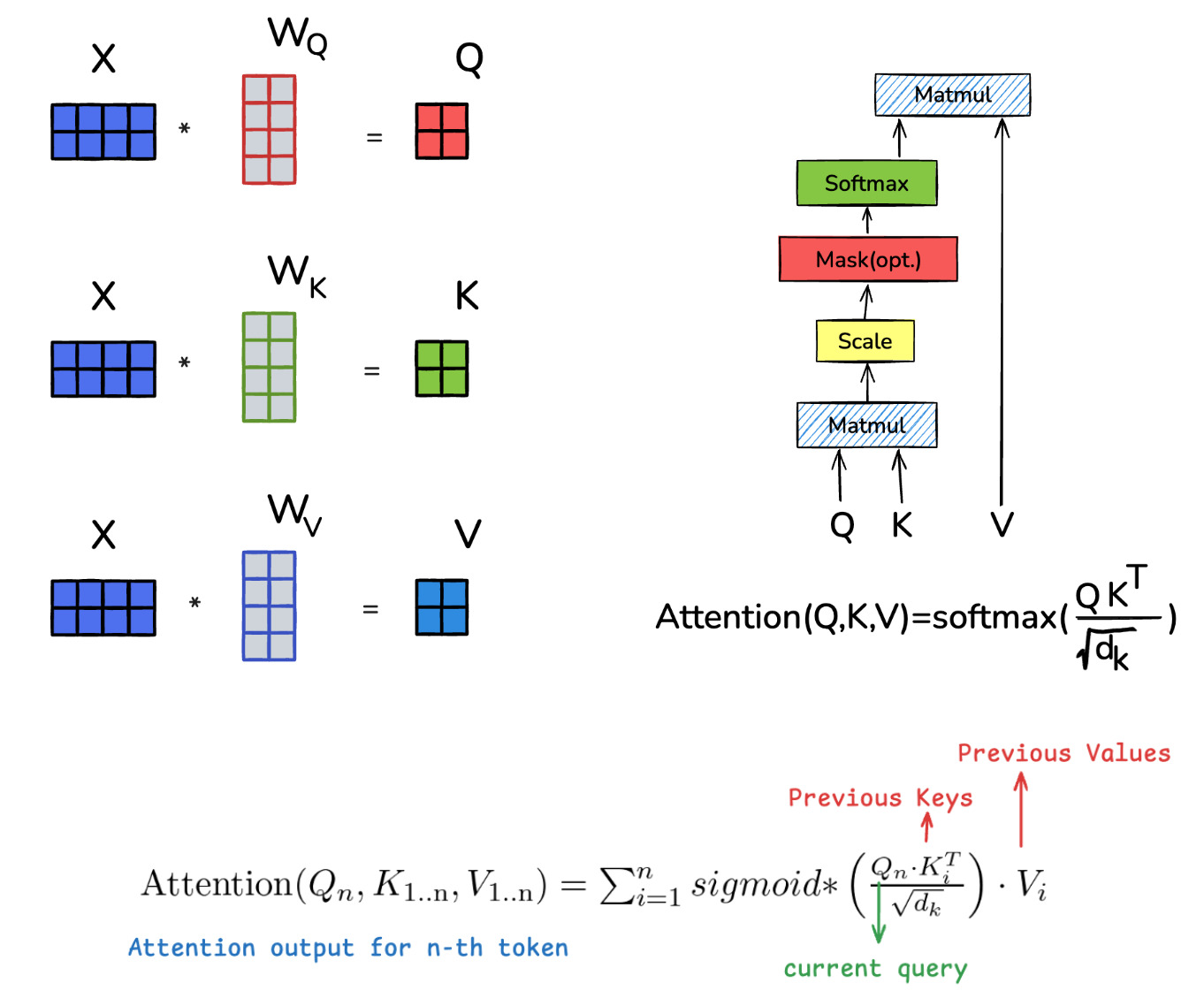Attention Math and Visualisation

Additional Modifications

We have mentioned that if there are q transformations $M_q$ and k transformations $M_k$, we can have $q * k$ different relationships. In general, initially, we had one transformation $M_k$ for every transformation $M_q$. This is called Multi Head Attention as introduced in Attention is all you need. But you can very well have a single transformation $W_k$ that is shared by all the $q$ transformations. This is called Multi Query Attention as introduced in Fast Transformer Decoding: One Write-Head is All You Need by none other than Noam Shazeer. But we can have a middle ground between the two where every set of g queries share the same key transformation. This is called Grouped Query Attention as introduced in the similarly named paper.

Generally speaking, you call each such relation an Attention Head, you denote the number of heads (query transformations) as $n_h$. The number of key transformations is denoted as $n_k$. The number of value transformations matches the number of key transformations.

If you’d like to read more about the differences, how they stack up, what are the tradeoffs, you can read my other blog Transformer Showdown.

This image from DeepSeek V2 paper gives a crisp view of the above mentioned architectures.

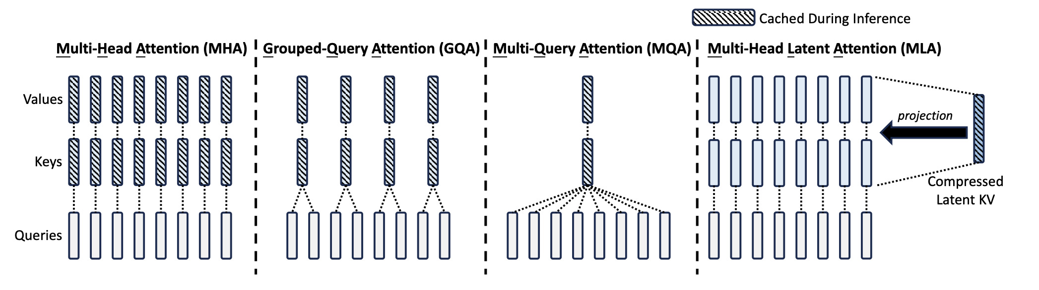MHA vs GQA vs MQA vs MLA

MLP or FFNN

So far so good. We have captured all the inter token relationships. There is still the task of ignoring or deleting all the unnecessary features and also in a certain way capturing the intra token relationships. To do that, we need to operate on the vectors individually. No more global operations. This is the job of the Feed-Forward Neural Network (FFNN), also called a Multi-Layer Perceptron (MLP).

The simplest way to do that is to have a linear transformation (yeah again :)). We can project the input from d to i dimensions. This is done by a matrix $M_i \in \mathbb{R}^{d \times i}$. i need not be related to d in any way. But there is one advantage of having i higher than d. It allows us to linearly seperate data in that higher dimension that wasn’t linearly separable in the lower dimension. You can watch this video for reference.

Note: Generally speaking, the intermediate dimension i is approximately 3-4 times the input dimension d. This is a good rule of thumb. In my small scale experiments, I found that 2-4x is a good choice. Anything lower or anything higher, the performance degraded.

Once separated, we can delete/remove those features that are not needed. Later we can project back onto the lower dimensions. We apply ReLU to the higher dimension output to remove the some of those features. ReLU is a function that is 0 for negative inputs and the input for positive inputs. $ReLU(x) = max(0, x)$. Note that if you don’t apply any non linearity, you can simply combine both the linear transformations into a single matrix.

$(X M_i) M_o == X (M_i M_o) == X (M) $ courtesy, associtivity of matrix multiplication.

So, we do the following:

\[\begin{align*} O &= X M_i && \in \mathbb{R}^{n \times i} \quad \text{ project to higher dimensions }\\ O &= \text{ReLU}(O) && \in \mathbb{R}^{n \times i} \quad \text{ apply non linearity }\\ O &= O M_o && \in \mathbb{R}^{n \times d} \quad \text{ project back to lower dimensions } \end{align*}\]

One small change you see in recent architectures is that there is another step before projecting onto lower dimensions. This is from Noam Shazeer’s work GLU variants improve Transformer. He himself mentions “These architectures are simple to implement, and have no apparent computational drawbacks. We offer no explanation as to why these architectures seem to work; we attribute their success, as all else, to divine benevolence.” who am I to argue anyway?

\[\begin{align*} O_g &= X M_g && \in \mathbb{R}^{n \times i} \quad \text{ gate projection }\\ O_u &= X M_u && \in \mathbb{R}^{n \times i} \quad \text{ up projection }\\ O &= (\text{SiLU}(O_g) \odot O_u) M_d && \in \mathbb{R}^{n \times d} \quad \text{ project back to lower dimensions } \end{align*}\]

The nomenclature

• $X$ is the input matrix.
• $M_q$ is the transformation matrix for the query. Denoted as $W_Q$ or q_proj in the code.
• $M_k$ is the transformation matrix for the key. Denoted as $W_K$ or k_proj in the code.
• $M_v$ is the transformation matrix for the value. Denoted as $W_V$ or v_proj in the code.
• $M_o$ is the transformation matrix for the output. Denoted as $W_O$ or o_proj in the code.
• $M_g, M_u, M_d$ are the transformation matrices for the FFNN layer. Denoted as $W_G, W_U, W_D$ or gate_proj, up_proj and down_proj in the code.
• $n_h$ is the number of heads.
• $n_k$ is the number of key/value transformations.
• $h$ is the dimension of the head.
• $d$ is the dimension of the output.
• $n$ is the number of words in the sequence.
• $i$ is the intermediate dimension.

Here’s an example of Llama 3 8B. (nn.Linear is the linear transformation matrix in PyTorch)

LlamaForCausalLM(
  (model): LlamaModel(
    (embed_tokens): Embedding(128256, 4096)
    (layers): ModuleList(
      (0-31): 32 x LlamaDecoderLayer(
        (self_attn): LlamaSdpaAttention(
          (q_proj): Linear(in_features=4096, out_features=4096, bias=False)
          (k_proj): Linear(in_features=4096, out_features=1024, bias=False)
          (v_proj): Linear(in_features=4096, out_features=1024, bias=False)
          (o_proj): Linear(in_features=4096, out_features=4096, bias=False)
          (rotary_emb): LlamaRotaryEmbedding()
        )
        (mlp): LlamaMLP(
          (gate_proj): Linear(in_features=4096, out_features=14336, bias=False)
          (up_proj): Linear(in_features=4096, out_features=14336, bias=False)
          (down_proj): Linear(in_features=14336, out_features=4096, bias=False)
          (act_fn): SiLU()
        )
        (input_layernorm): LlamaRMSNorm()
        (post_attention_layernorm): LlamaRMSNorm()
      )
    )
    (norm): LlamaRMSNorm()
  )
  (lm_head): Linear(in_features=4096, out_features=128256, bias=False)
)

Finishing notes

We have looked at the attention mechanism and motivated the reasoning behind it and why is the way it is. We have also peeked into the MLP, positional encodings, residual connections, and the final output layer. The motive of this conversation was to spike the curiosity and get you to read more about the topic. We still haven’t talked about Embeddings in detail, different types of normalisation etc. Those are all very interesting topics in themselves and we might cover them if there’s enough interest. But for now, I’ll leave you with a couple of questions that probably motivates you to learn more.

1. How do you differentiate between “A defeated B” and “B defeated A”?
2. How do you predict the word given a vector representation of the word aka go from $d$ dimensional vector to the word?
3. How are the weights $W_x$ initialised? What are the implications of initialising them around 0?

With that, I’ll end this conversation. Thank you for reading. If you have any comments, concerns, questions, or suggestions, please feel free to reach out to me. You can find me on LinkedIn or Twitter.