Transformer showdown MHA vs MLA vs nGPT vs Differential Transformer
Comparing various transformer architectures like MHA, GQA, Multi Latent Attention, nGPT, Differential Transformer.
Transformer Showdown
For a long time, I had the urge to understand what advantages each of the changes to transformer architecture gives. I created a small repo that I like to call nanoformer where I compare various architectures like MHA, GQA, Multi Latent Attention, nGPT and Differential Transformer. Switching between the mentioned architectures is as easy as modifying a CLI argument. So without further ado, lets get comparing.
Attention variants:
Multi Head Attention (MHA)
The standard attention that was introduced as part of Attention is all you need. Very commonly used in a lot of models before 2023. Each layer has equal number of query, key and value heads. So if a layer has
\[Q_i = W_{q_i} X, \quad K_i = W_{k_i} X, \quad V_i = W_{v_i} X \quad \text {where X is the input}\] \[Q = [Q_1, Q_2,..., Q_h], \quad K = [K_1, K_2,..., K_h], \quad V = [V_1, V_2,..., V_h] \quad \text {where [ ] is concatenation}\] \[A_i = \text{Attention}(Q_i, K_i, V_i) = softmax(\frac{Q_iK_i^T}{\sqrt{d_k}})V_i\] \[A = [A_1, A_2, ..., A_h] \space @ \space Wo\]hheads, we’d havehqueries,hkeys andhvalues.Config :
nlayers. Each layer hashheads. Each head hasddimensions. Total token countt.Parameters: \(W_{q_i}\) is of shape \((h*d, d)\), so has \(h*d^2\) parameters per head. Same for \(W_{k_i}, W_{v_i}\). So \(W_q + W_k + W_v\) contributes to a total of \(3*h*(h*d^2)\) paramters. \(W_o\) is of size \((h*d, h*d)\) so \(h^2*d^2\) parameters. Total of \(4*n*h^2*d^2\).
For example, Llama-2-7b-hf has 32 attention heads and 32 key value heads. So llama 2 7B uses MHA. It has a hidden_size of 4096. This means, each head has a head_dim (d) of 128. So the algebra tells us that \(W_{q_i}\) would be of shape \((128 *32,128) = (4096,128)\). Each Q (similarly K,V) would be of shape \((4096, 128*32)=(4096,4096)\) contributing to \(128^2 * 32^2=16,777,216\) paramters. Executing the below code would give you the same result. Voila.
1
2
3
4
5
6
7
8
9
10
11
12
13
14
15
16
17
18
19
20
21
22
  llama2 = AutoModelForCausalLM.from_pretrained(
      'meta-llama/Llama-2-7b-hf',
      device_map='cuda:0',
      torch_dtype = torch.bfloat16,
  )

  q_shape = llama2.model.layers[0].self_attn.q_proj.weight.shape
  q_params = llama2.model.layers[0].self_attn.q_proj.weight.numel()

  k_shape = llama2.model.layers[0].self_attn.k_proj.weight.shape
  k_params = llama2.model.layers[0].self_attn.k_proj.weight.numel()

  v_shape = llama2.model.layers[0].self_attn.v_proj.weight.shape
  v_params = llama2.model.layers[0].self_attn.v_proj.weight.numel()

  o_shape = llama2.model.layers[0].self_attn.o_proj.weight.shape
  o_params = llama2.model.layers[0].self_attn.o_proj.weight.numel()

  print(f'Wq shape is {q_shape} contributes to {q_params} paramters')
  print(f'Wk shape is {k_shape} contributes to {k_params} paramters')
  print(f'Wv shape is {v_shape} contributes to {v_params} paramters')
  print(f'Wo shape is {o_shape} contributes to {o_params} paramters')
1
2
3
4
  Wq shape is torch.Size([4096, 4096]) contributes to 16777216 paramters
  Wk shape is torch.Size([4096, 4096]) contributes to 16777216 paramters
  Wv shape is torch.Size([4096, 4096]) contributes to 16777216 paramters
  Wo shape is torch.Size([4096, 4096]) contributes to 16777216 paramters
Activations: Each token’s query is of size
d(per head). The same is for key and value. Hence a total of \(3*n*h*d\) per token. The final output is of same shape as well. The attention scores, one per each pair of input tokens, form a matrix of size \(t*t\) hence \(t^2\). So a total of \(4*n*h*d*t + n*h*t^2\).KVCache: Each key and value is of size
dper token per head per layer. Hence a total of \(n*h*d*t\) for key (and value). So the size of KV Cache is \(2*n*h*d*t\)Multi Query Attention (MQA)
A small modification of MHA. Instead of having one key and value per query head, we’d only have a single key per token and all the query heads try to find similarity with that. This results in each layer having
\[A_i = \text{Attention}(Q_i, K, V_i) = softmax(\frac{Q_iK^T}{\sqrt{d_k}})V_i\] \[A = [A_1, A_2, ..., A_h] \space @ \space Wo\]hqueries,1key and1value. The advantage here is that if you’re saving KVCache for speeding up inference, your KVCache is reduced byhtimes. But this is not as performant as MHA as we’re reducing the scope of information stored in keys to only single vector.- Parameters: \(W_{q_i}\) is of shape \((h*d, d)\), so has \(h^2*d^2\) parameters. As for \(W_{k_i}, W_{v_i}\), they output a single vector per head. So \((d,d)\) shape and hence \(d^2\) parameters. \(W_o\) is of size \((h*d, h*d)\) so \(h^2*d^2\) parameters. Total of \(2*n*h^2*d^2 + 2*n*h*d^2\).
- Activations: Each token’s query is of size
d(per head) So \(h*d\).There is only one key shared across all the heads hence only \(2*d\) (key and value). Hence a total of \(n*h*d*t + 2*n*d*t\). The final output is of same shape as query as well. The attention scores form a matrix of size \(t*t\) hence \(t^2\). So a total of \(2*n*h*d*t + 2*n*d*t + n*h*t^2\). - KVCache: Each key and value is of size
dper token per layer. Hence a total of \(2*n*d*t\). A compression ofhtimes compared to MHA.
Grouped Query Attention (GQA)
This acts as a middle ground between MHA and MQA. Instead of 1 key and value catering to all the queries, we have 1 key and value catering to a group of queries. So we’d have
\[A_i = \text{Attention}(Q_i, K_{i//g}, V_i) = softmax(\frac{Q_iK_{i//g}^T}{\sqrt{d_k}})V_i\] \[A = [A_1, A_2, ..., A_h] \space @ \space Wo\]hqueries,kkeys andkvalues wherekdividesh. So for each layer, you’d be storing2 * kembedding vectors. You’d find a lot of models that use this architecture. Generally speaking, a single query caters to4to8queries. You can identify whether a model uses this when you seenum_attention_heads≠num_kv_headsin model’s config.jsonParameters: \(W_{q_i}\) is of shape \((h*d, d)\), so has \(h^2*d^2\) parameters. As for \(W_{k_i}, W_{v_i}\), they output a single vector per group of heads. So \((g*d,d)\) shape and hence \(g*d^2\) parameters. \(W_o\) is of size \((h*d, h*d)\) so \(h^2*d^2\) parameters. Total of \(2*n*h^2*d^2 + 2*n*g*h*d^2\).
1
2
3
4
5
6
7
8
9
10
11
12
13
14
15
16
17
18
19
20
21
  llama3 = AutoModelForCausalLM.from_pretrained(
      'meta-llama/Meta-Llama-3.1-8B-Instruct',
      device_map='cuda:0',
      torch_dtype = torch.bfloat16,
  )
  q_shape = llama3.model.layers[0].self_attn.q_proj.weight.shape
  q_params = llama3.model.layers[0].self_attn.q_proj.weight.numel()

  k_shape = llama3.model.layers[0].self_attn.k_proj.weight.shape
  k_params = llama3.model.layers[0].self_attn.k_proj.weight.numel()

  v_shape = llama3.model.layers[0].self_attn.v_proj.weight.shape
  v_params = llama3.model.layers[0].self_attn.v_proj.weight.numel()

  o_shape = llama3.model.layers[0].self_attn.o_proj.weight.shape
  o_params = llama3.model.layers[0].self_attn.o_proj.weight.numel()

  print(f'Wq shape is {q_shape} contributes to {q_params} paramters')
  print(f'Wk shape is {k_shape} contributes to {k_params} paramters')
  print(f'Wv shape is {v_shape} contributes to {v_params} paramters')
  print(f'Wo shape is {o_shape} contributes to {o_params} paramters')
1
2
3
4
  Wq shape is torch.Size([4096, 4096]) contributes to 16777216 paramters
  Wk shape is torch.Size([1024, 4096]) contributes to 4194304 paramters
  Wv shape is torch.Size([1024, 4096]) contributes to 4194304 paramters
  Wo shape is torch.Size([4096, 4096]) contributes to 16777216 paramters
Activations: Each token’s query is of size
d(per head) resulting in \(h*d\) sized tensor. There is one key per group of heads hence only \(d*g\) (key, value) which together add up to \(2*d*g\) per token. Hence a total of \(n*h*d*t + 2*n*g*d*t\). The final output is of same shape as query as well. The attention scores form a matrix of size \(t*t\) hence \(t^2\). So a total of \(2*n*h*d*t + 2*n*g*d*t + n*h*t^2\).KVCache: Each key and value is of size
dper token per layer per group. Hence a total of \(2*n*g*d*t\). A compression ofh/gtimes compared to MHA.MultiHead Latent Attention (MLA)
A new architecture found in DeepSeek V2 family of models. Here, we compress the Keys and values into a latent space and uncompress them back to original space when inference takes place. The idea is to get the advantages of MHA while saving up on KVCache as it scales linearly with context length. Each key and value are compressed from
ddimensions tocdimension space.Last year, I was playing around with llama 2 and mistral family of models. I tried to understand why some models perform better than the others from a mathematical perspective. I was fiddling with eigen values of each of the weight matrices. What I observed was very interesting. All the models exhibit some sort of low rank behaviour, where 50% of the eigen values explain 90% of the variance (Read for reference). So essentially, we can compress the keys and values (evne queries) to atleast half their original size without losing much information. This can be thought of as an explanation to why MLA might work. The compression ratio is higher than 2:1 but you get the idea.
\[c_t^{KV} = W^{DKV} X, \quad \text{ where } c_t^{KV} \in \mathbb{R}^{c} \quad \text { is down projection of keys }\] \[k_t^C = W^{UK} c_t^{KV} \quad \text { up projection of keys}\] \[v_t^C = W^{UV} c_t^{KV} \quad \text { up projection of values}\] \[c_t^{Q} = W^{DQ} X \quad \text{ where } c_t^{Q} \in \mathbb{R}^{c}\] \[q_t^C = W^{UQ} c_t^{Q}\] \[A_i = \text{Attention}(Q_i, K_i, V_i) = softmax(\frac{Q_i K_i^T}{\sqrt{d_k}})V_i\] \[A = [A_1, A_2, ..., A_h] \space @ \space Wo\]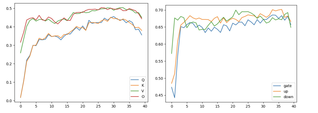 Share of eigen values contributing to 90% in weight
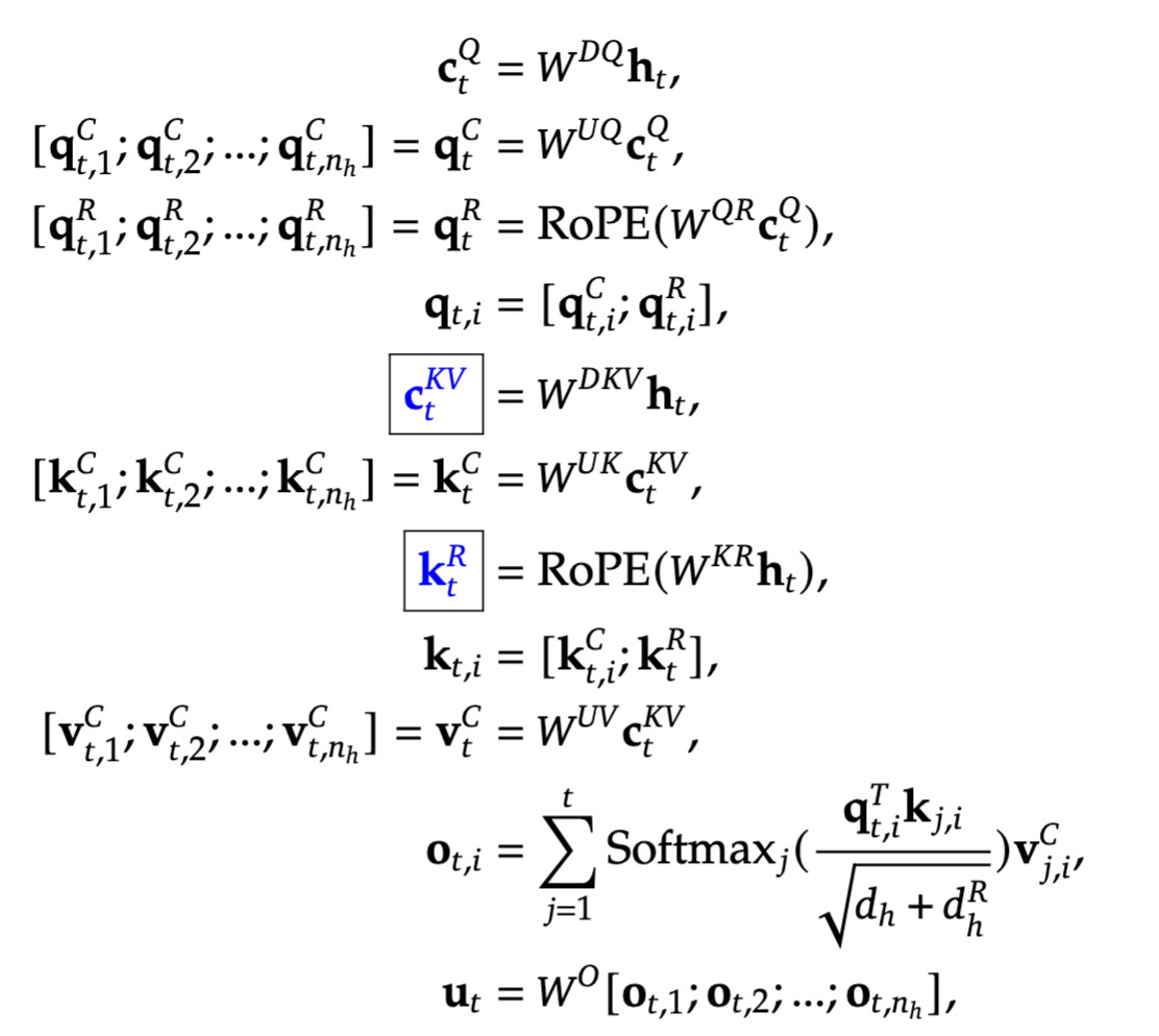 Multi Latent Attention formulae
KVCache: Each compressed vector is of size
cper token per layer per group. Hence a total of \(n*g*c*t\). Keys and values are inferred by decompressing this (\(k_t^C, v_t^C\)). A compression of2*d/ctimes compared to MHA. Note that in final implementation there’s a nuance of additional heads (and hence keys and values) for RoPE. That adds a little more overhead. So the compression ratio essentially becomes \(2*d/(c+r)\) where r is the RoPE key dimension.
This image from DeepSeek V2 paper gives a crisp view of the above mentioned architectures.
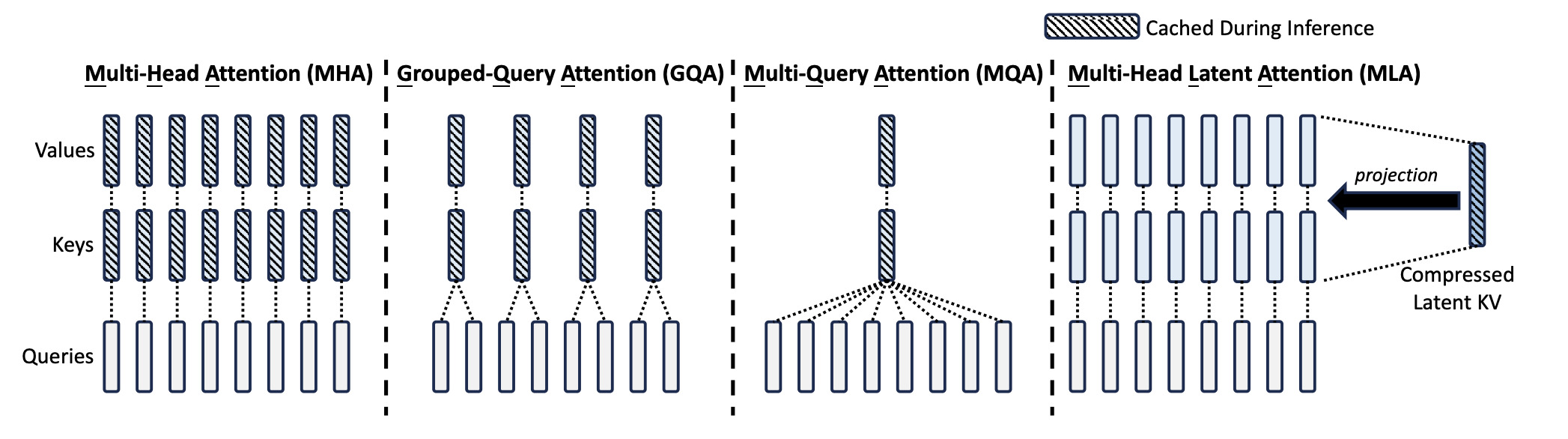 MHA vs GQA vs MQA vs MLA
Other Transformer Variants:
Differential Transformer
Introduced in a 2024 paper from Microsoft. The main motivation is that attention scores have a lot of noise. So if we have two subnetworks calculating attention, subtracting one from the other would act as subtracting random noise from information induced with noise. This helps control the attention scores and logits (outliers are of lesser magnitude). This is said to improve convergence. We discussed this in great detail in one of our other blogs on substack, check it out.
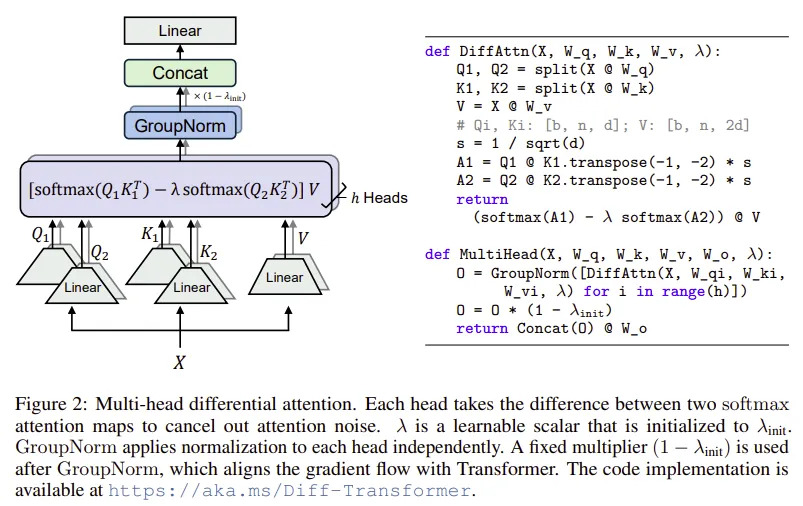 Differntial Transformer
- Even though attention units, each attention head is half the dimension as original, so the number of paramters, activations and KVCache requirement is the same as that of GQA.
nGPT
Introduced in a 2024 paper from NVIDIA. The main idea is, if normalisation layers are so important to the performance of deep networks and LLMs, why not make normalistion mathemtically implicit to the network. Given this assumption, at every step, we try to make sure we’re interacting with normalized vectors and only normalised vectors are passed on after every step. This too is said to improve convergence. We discussed this in great detail in one of our other blogs on substack, check it out.
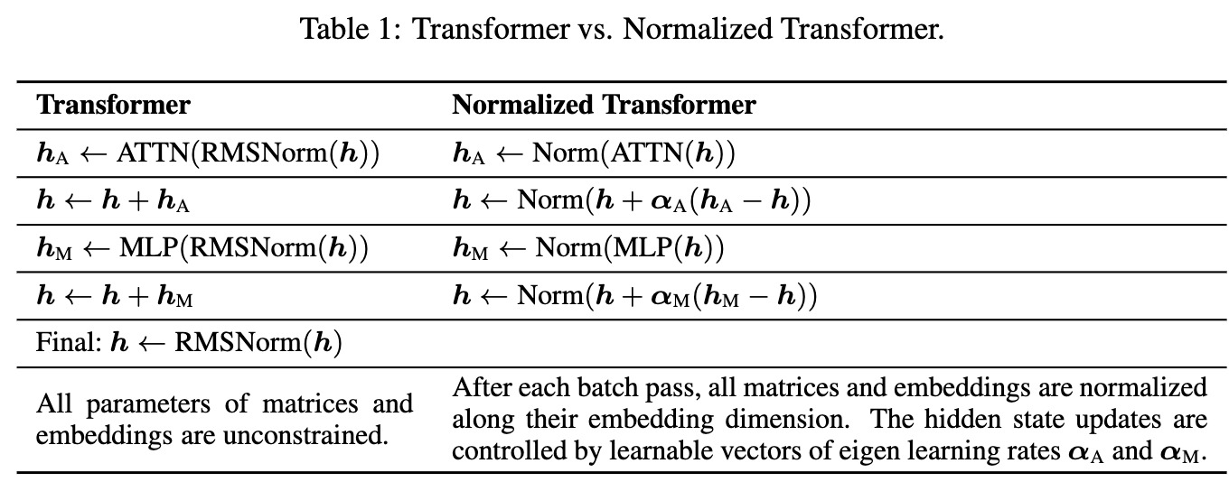 nGPT formulae
- Apart from more normalisations there isn’t much that would meaningfully contribute to parameters or activations or KVCache as compared to GQA.
Results and Findings
So now that the introductions are out of the way, the burning question is do the changes contribute to any meaningful differences in the final performance of the models?
Well the answer is nuanced. Let’s see how they stack up.
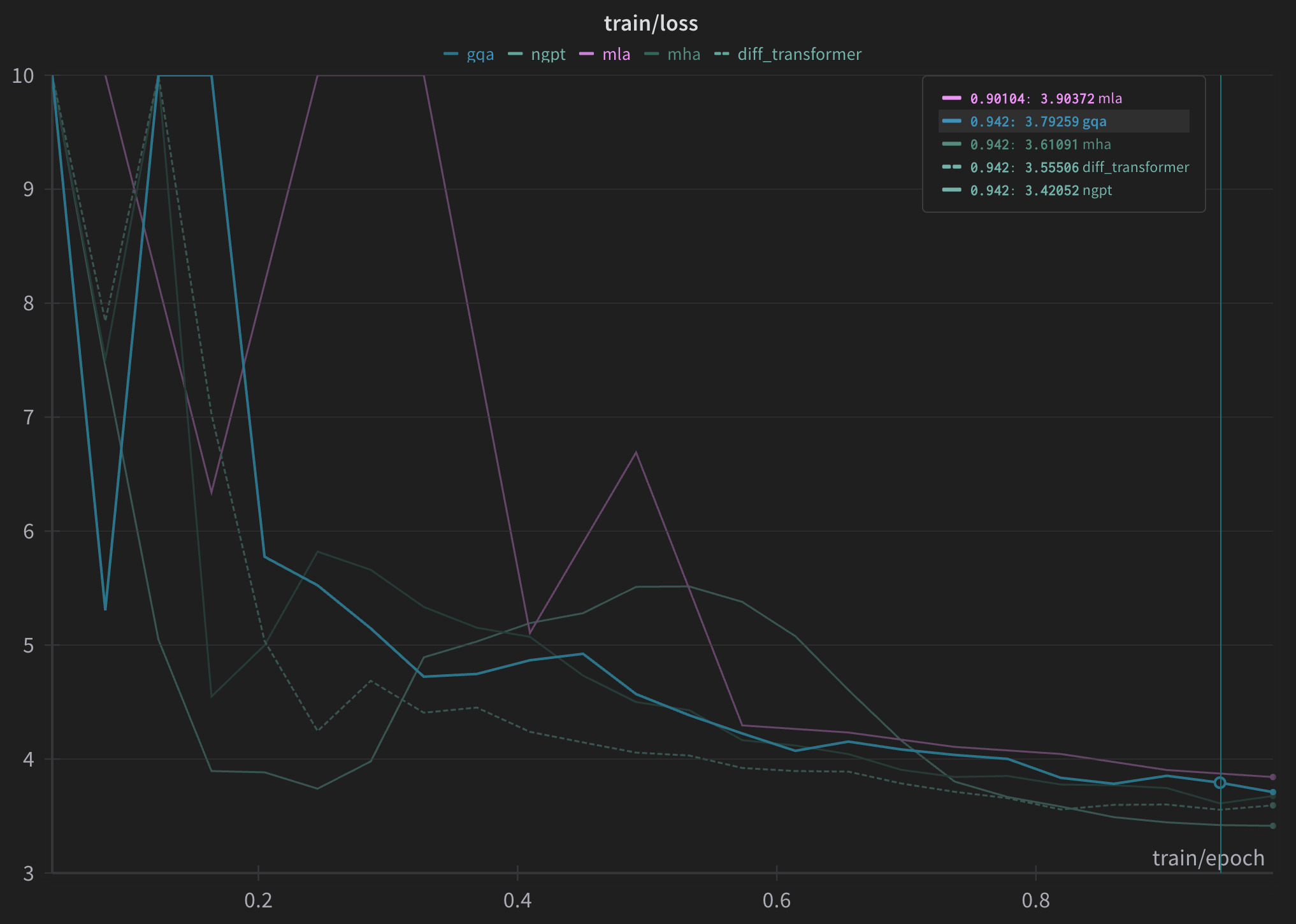 Train losses on wikipedia dataset
I started with a model that has 16 layers, with a hidden size of 1536. The MHA variant had 16 attention heads (hence 16 key value heads) while the GQA variant had 4 key value heads. The MLP block had an intermediate size of 2048. I used GPT2 tokenizer from NeelNanda which is modified to treat numbers as individual tokens.
Looks like nGPT outperforms the rest by a decent margin on a 100k sample of the wikipedia dataset
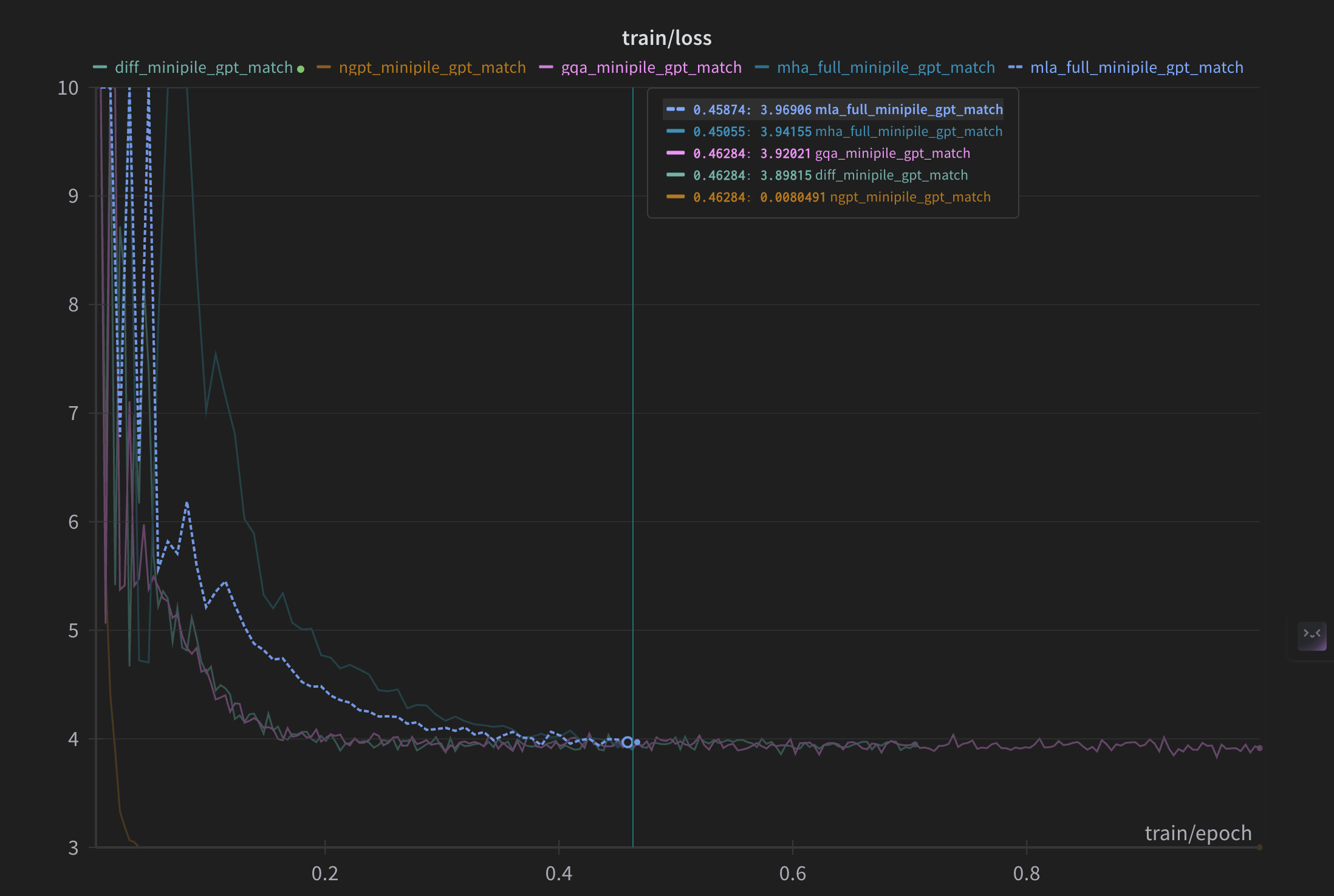 Train losses on minipile dataset
On the minipile dataset which is approximately 10x larger than the wiki data, I saw that there isn’t much to choose between MLA, MHA, GQA and DiffAttention. Which is great since GQA uses 4x less keys and values resulting in 4x less KVCache. Surprisingly, nGPT’s losses seem to go down as low as 0.2 when the others hover around 3. I tried to repeat the experiement multiple times with multiple configs only to find a similar loss curve. I also checked validation loss for all the models, they look very similar to train loss curves so there isn’t much value in plotting those. We will have to look into why this is the case but it definitely is fascinating.
Conclusion
All in all, GQA offers a very good alternative to MHA, sometimes even outperforming it while also using 4-8x less space for KVCache. MLA builds upon that by compressing the Keys and values even further. Turns out, this also acts as regularisation. Normalisation is the king of all. Given that normalisation is a key component in deep learning, it is no surprise that making it explicit for every operation. This opens up new paths to LLM training. We will explore the down stream capabilities of the models in a future write up. Until then, Ciao.