Understanding multi GPU Parallelism paradigms

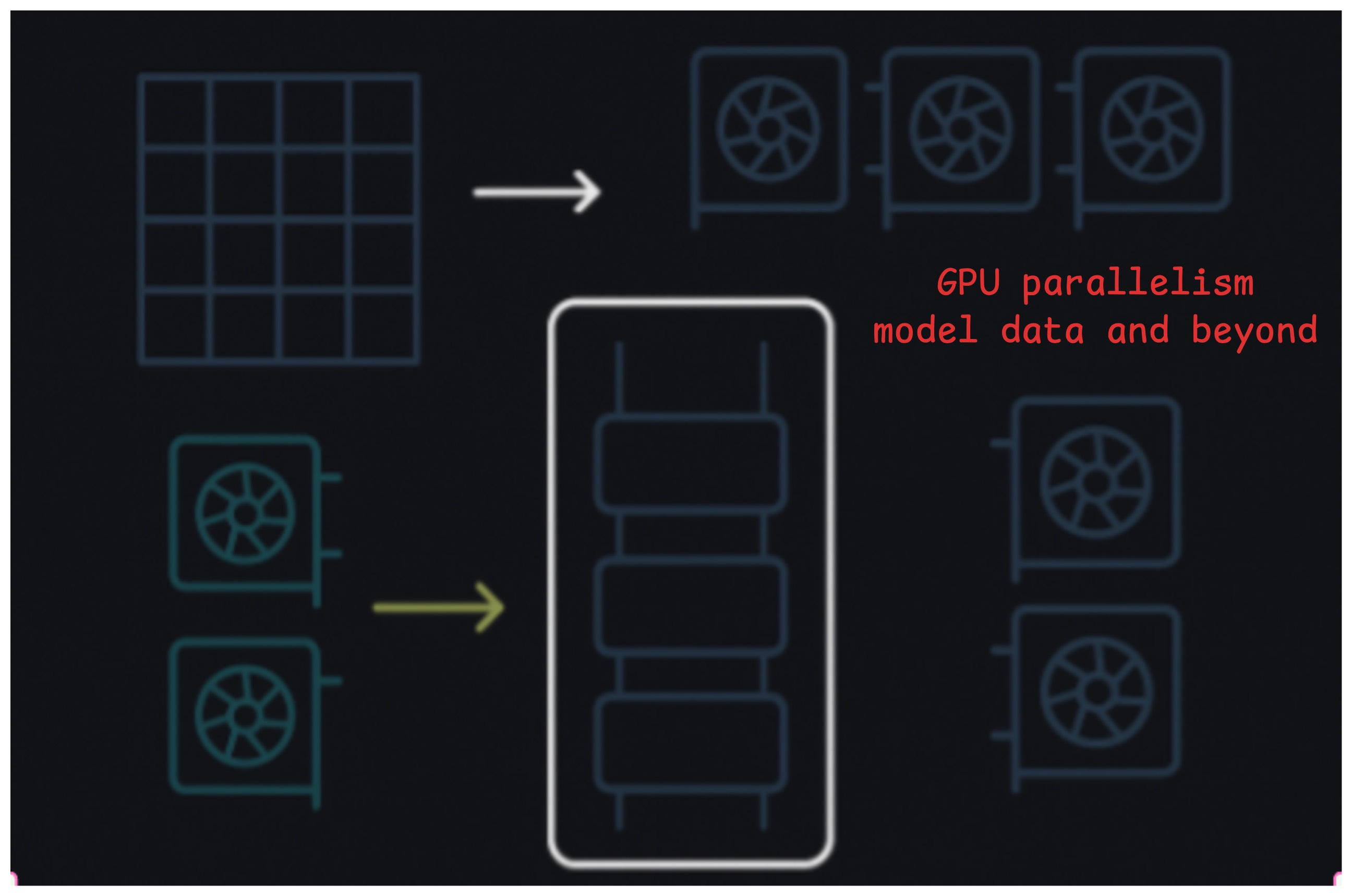
We’ve been talking about Transformers all this while. But how do we get the most out of our hardware? There are two different paradigms that we can talk about here. One case where your model happily fits on one GPU but you have many GPUs at your disposal and you want to save time by distributing the workload across multiple GPUs. Another case is where your workload doesn’t even fit entirely on a single GPU and you need to work that around. Let’s discuss each of these in a little more detail. We will also try to give analogies for each of the paradigm for easier understanding. Note that anytime we mention GPU or GPUx hereon, you can safely replace it with any compute device. It can be GPU or TPU or a set of GPUs on single node etc.

Data Parallelism

Say you have to carry boxes of items, each of 2Kg from point A to point B which are say 2Km apart. Assume that you have enough energy to do the entire job by yourself. But you have two copies of you. So your first copy and second copy operate together, carry 4Kg from A to B in the same time either of you would’ve carried 2Kg. This is data parallelism. The key is that you alone can carry 2Kg for 2Km so your capacity is 2Kg * 2Km = 4KgKm per replica of you

This is the case where your workload fits entirely on a single GPU. So you essentially run copies of the workload. So if you’re trying to do inference, we have replicas so that inference requests are distributed across the GPUs. So in any given instant, your “system” can process n times more requests if you have n GPUs. Your throughput went up by n times :)

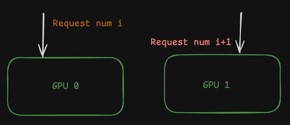Data Parallel Inference

Another case of this is for training. If you can fit the entire training components (aka model weights, activations, gradients and optimiser states) onto single GPU for a given batch size, you can essentially simulate a larger batch size by utilising multiple GPUs. So first few samples (1-16 in the image) have their forward and backward pass on GPU0 and the rest (17-32 in the image) have their forward and backward pass on GPU1. So in theory, if your workload needs 1000 GPU hours for training your model, instead of running it on single GPU for 1000 hours, you can do training on 10 GPUs for 100 hours. So you’re saving a lot of wall clock time.

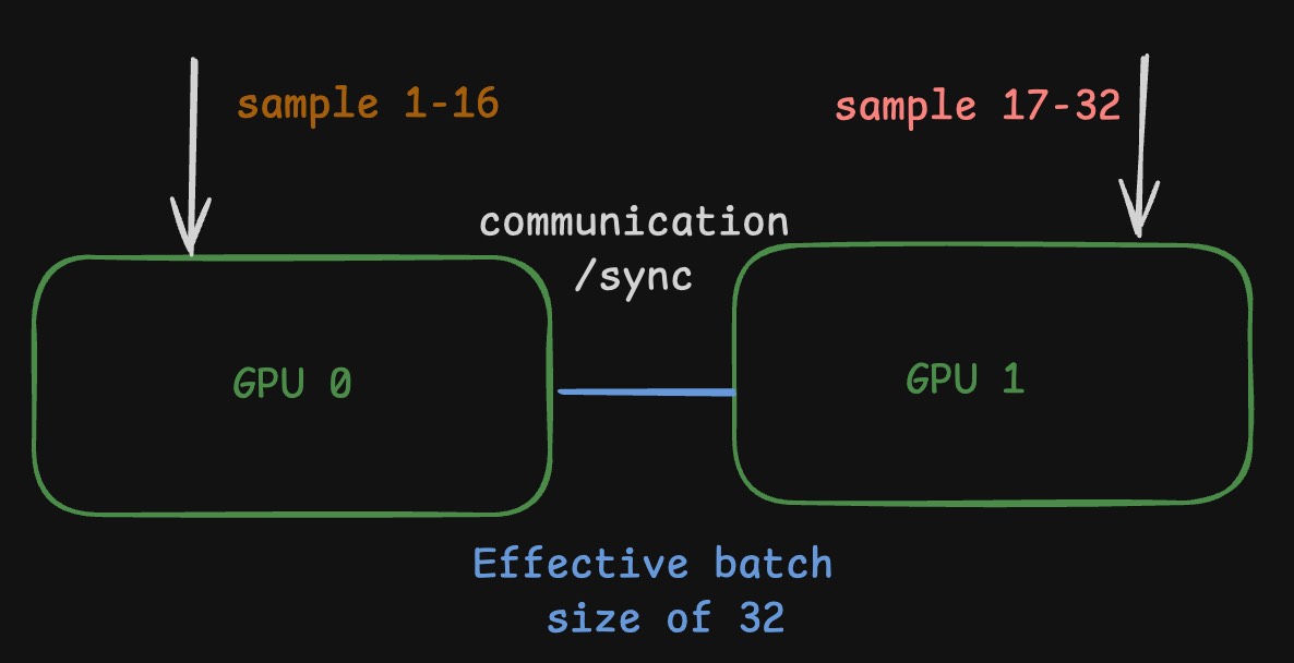Data Parallel Training

Do note that this is a gross over simplification. We’d need a lot of things to be done right like moving gradients and syncing weights across GPUs/nodes. But that is beyond the scope of this blog.

Model Parallelism

All is good when you can fit model and workload onto a single GPU. But what if you cannot? Models are growing in size day by day. You can’t possibly fit them in single GPU. More so with increasing context lengths everyday. So what do you do? You essentially split the model across GPUs. That is what we call Model Parallelism. We’ll talk about how it is done in a little more detail.

Pipeline Parallelism

Now what if you can’t carry 2Kg for a distance of 2Km? But you can only do 2Kg for 1Km and you’d be exhausted. aka your capacity is 2Kg*1Km = 2KgKm. What you’d do is have the other copy of yourself at a midpoint C which is 1Km from either end, carry the box over to C, hand it over to your replica and let them carry it from C to B for the last 1Km. (Assume that you’d magically teleport to A from C and replenish your energy. Cartoon physics or something)

This is where you split the pipeline into two parts. So for example, if you have transformer with 32 layers, you might load first half aka 1-16 layers on GPU0 and second half aka 17-32 layers on GPU1. This way, when you are passing input through the model, it first goes through GPU0, the intermediate output is then passed through to GPU1 and the rest of the computation is done on GPU1. The final output is then returned as shown in the image.

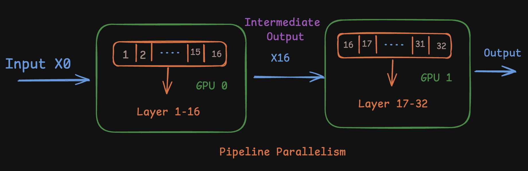Pipeline Parallel

This can be done both for inference and training, everything remains the same. Only thing we need to pass between GPUs here is the intermediate activations in case of inference. In case of training we might want to pass the gradients from GPU1 to GPU0 for back propogation. But nothing comes for free, this while being great for reducing inter GPU communication, takes a hit at GPU utilisation. So while GPU0 is processing the input, GPU1 is idle and vice versa. This gap is called bubble. It is critical to ensure that bubbles are minimised while relying on pipeline parallelism.

For inference, if you have continuous stream of requests, at some point in time, you’d have GPU0 processing batch n while GPU1 would be processing the previous batch aka batch n-1. In the next time step, once GPU0 is done with batch n (meanwhile GPU1 is done with batch n-1), GPU1 can pick it up and finish processing and this stream continues. Thus utilisation of both the GPUs is maxxed out. But this is an optimistic scenario. And you’d ideally need separate queues for both GPUs to make sure they don’t run Out of Memory while processing the inputs. Also there is very minimal hit to latency as compared to single GPU inference. The only additional step is transfering intermediate output between the GPUs once per forward pass. This is like you dropping the boxes at C and not worrying whether your replica would pick it up or not, while you have your own set of boxes waiting for you at A.

For training, there are different techniques to reduce pipeline bubbles. One should be wary of the fact that the order of backward pass is reverse of the order of forward pass. If forward pass starts at layer 1 and ends at layer 32, backward pass starts at layer 32 and ends at layer 1. So you can smartly design pipelining strategies to make the most out of the constrained setting we’re dealt with.

Tensor Parallelism

But in the previous case, while one replica was working, the other one was waiting on. But what if you want both of you to work at the same time? Assume that the boxes of 2Kg can be split into smaller boxes of 1Kg each so your capacity of 2KgKm can be distributed across 1Kg box and 2Km distance. In such a case, both of you would pick up the 1Kg boxes and start walking from A to B together. But this adds a constraint that even if one of the replicas finish earlier than the other, for the task to be complete, we need both smaller boxes. So the ideal case is to distribute the workload equally.

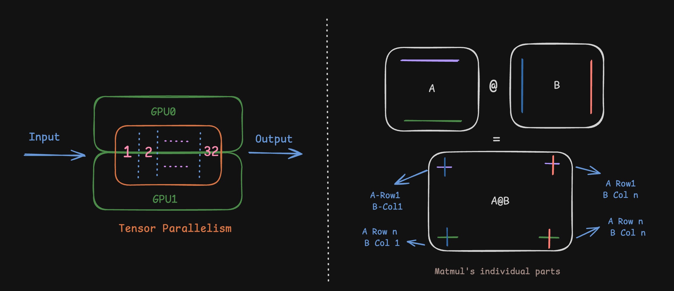
While pipeline parallelism splits the model across its depth, we can choose do the other splitting aka across its width. Doing this, every layer has its presence on both GPU0 and GPU1 (or across all n GPUs). Something that helps us heavily here is the fact that Matrix Multiplication, the most prominent operation in Deep Learning has parts which are independent of each other. We’ll see how this is done mostly from a matmul standpoint. Say you want to multiply two matrices A and B together. As shown in the image below, the result A@B (shape in the bottom), the element at index 1,1 depends on row 1 of A and column 1 of B. Similarly the element at index i,j depends only on row i of A and column j of B. The matrices can be any of Weights, Inputs, Intermediate results in the computation graph. The concepts still hold the same.

Tensor Parallel

If you recall, Mathematically speaking, if the matrix A is $[a_{ij}]$ and B is $[b_{ij}]$, we have $C = A@B$ and $C = [c_{ij}]$ where $c_{ij} = \sum_{k} a_{ik} \cdot b_{kj}$

Column Parallel

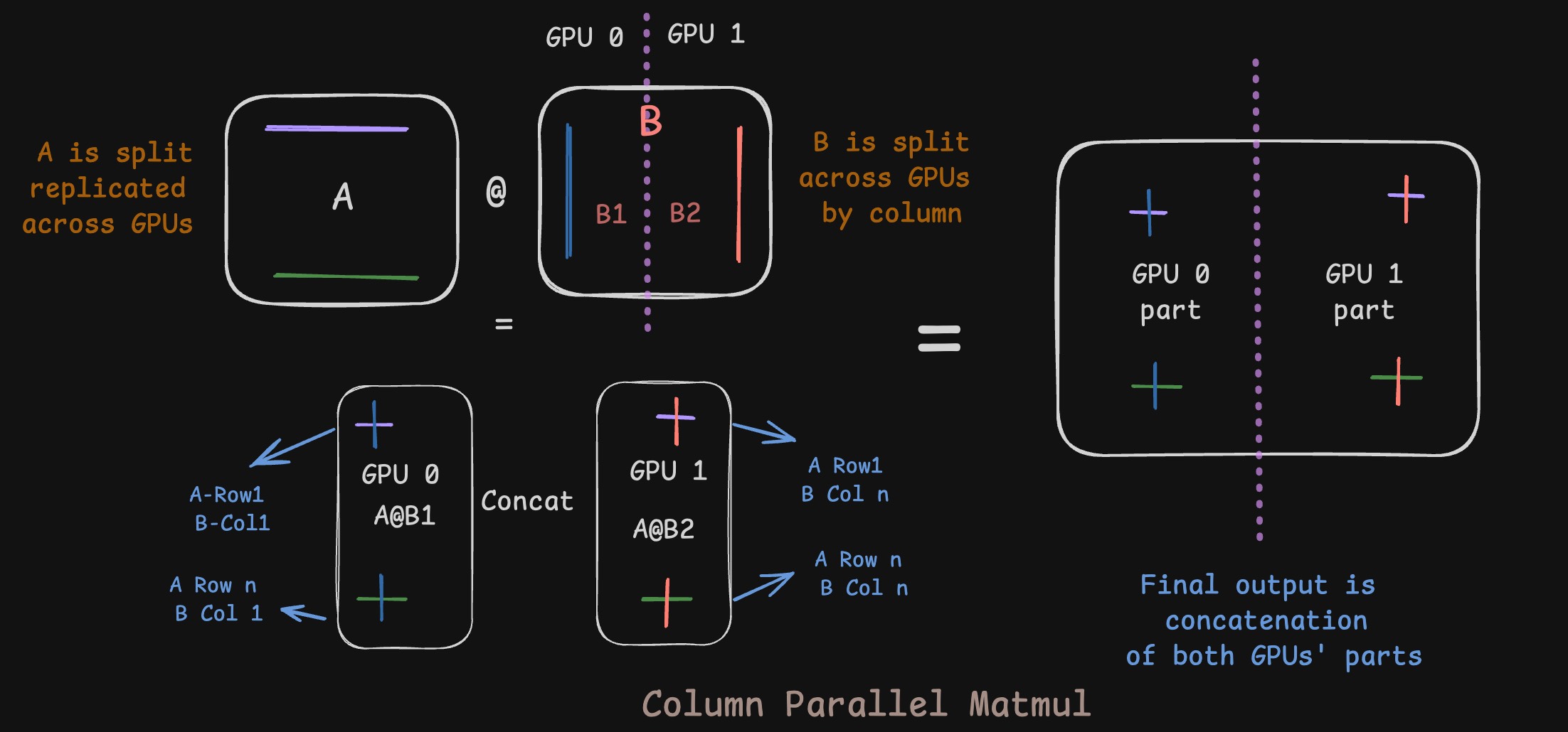
Given that we want to split model weights across GPUs, and that weight is a 2D matrix in general, we have two axes to split across. In the above example, if we split B across its columns, that will be called Column Parallel. In such a case, we’d replicate A across GPUs. The first few columns of the output would end up on GPU0 and the last few would end up on GPU1. If you want the entire output, you might have to concatenate the parts that are split across the GPUs.

Column Parallel

Mathematically, let’s denote the dimensions of the matrices with subscripts. If we have \(A_{m \times k}\) and \(B_{k \times n}\), the output \(C_{m \times n}\) is computed as follows. We split \(B\) along its columns into \(B_1\) and \(B_2\) for a 2-GPU setup, while replicating \(A\) on both:

\[C_{m \times n} = A_{m \times k} \cdot B_{k \times n} = A_{m \times k} \cdot \underbrace{\begin{bmatrix} (B_1)_{k \times n/2} & (B_2)_{k \times n/2} \end{bmatrix}}_{\text{B split by column}}\]

Since matrix multiplication distributes over blocks, we get: \(C_{m \times n} = \begin{bmatrix} \underbrace{(A \cdot B_1)_{m \times n/2}}_{\text{Computed on GPU0}} & \underbrace{(A \cdot B_2)_{m \times n/2}}_{\text{Computed on GPU1}} \end{bmatrix}\)

The final output is a simple concatenation of the results from each GPU.

Let’s look at the element-level calculation. An element \(c_{ij}\) is the dot product of row i from A and column j from B: \(c_{ij} = \sum_{k} a_{ik} \cdot b_{kj}\).

In Column Parallelism, the summation over k is never split. Each GPU computes the full dot product for a specific set of columns j.

• For $c_{1,1}$ (top-left) & $c_{m,1}$ (bottom-left): These are computed entirely on GPU0. \(c_{1,1} = \underbrace{\sum_{k} a_{1k} \cdot b_{k1}}_{\text{GPU0}} \quad , \quad c_{m,1} = \underbrace{\sum_{k} a_{mk} \cdot b_{k1}}_{\text{GPU0}}\)
• For $c_{1,n}$ (top-right) & $c_{m,n}$ (bottom-right): These are computed entirely on GPU1. \(c_{1,n} = \underbrace{\sum_{k} a_{1k} \cdot b_{kn}}_{\text{GPU1}} \quad , \quad c_{m,n} = \underbrace{\sum_{k} a_{mk} \cdot b_{kn}}_{\text{GPU1}}\)

And for those of you who prefer to speak the language of computers, you can verify it by doing

import torch
m,n,k = 4,4,4
# initialise random matrices
A = torch.randn((m,k))
B = torch.randn((k,n))
O = A@B # original computation
# split B column wise
B1 = B[:,:n//2]
B2 = B[:,n//2:]
# use the same A for both splits of B
O1 = A@B1
O2 = A@B2
# concatenate the output
O_split_concat = torch.cat((O1, O2), dim=-1)
# verify that the results are equal
assert torch.allclose(O, O_split_concat), "The results are not equal. Something went wrong"

Row Parallel

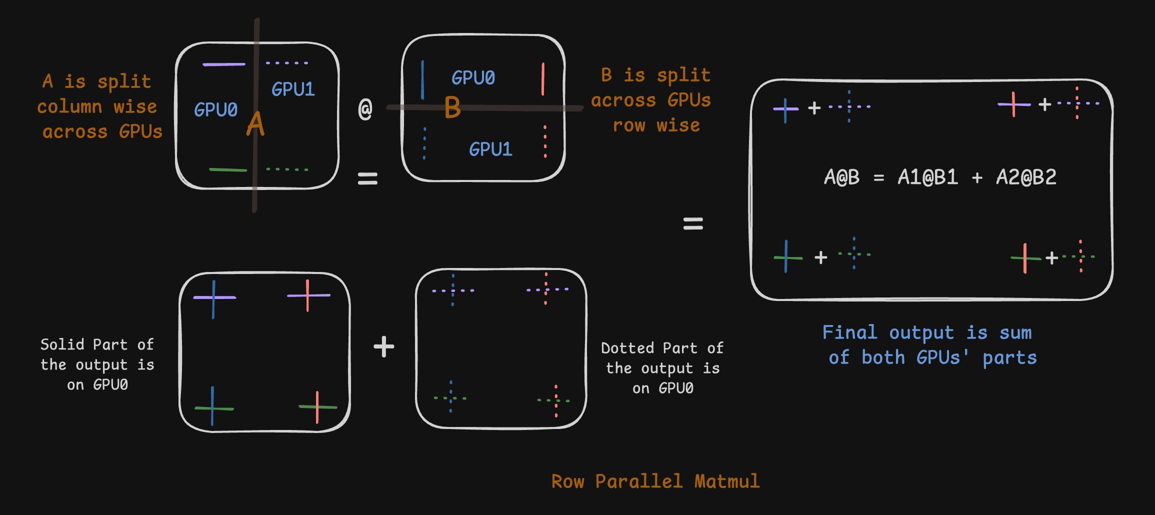
The counterpart to Column Parallel is rightly Row Parallel. Here, we split B across its rows. In such a case, we’d split A column wise. Some computation of the dot product or multiplication would be done on GPU0 and the rest would be done on GPU1. The final output would be sum of the outputs generated across GPUs. Do remember that first k elements of any row of A interact with only the first k elements of any column of B (or any similarly indexed set of elements for that matter). So splitting B column wise, you’d naturally gravitate to splitting A row wise to maintain that relationship and avoid GPU communication.

Side note: We can in theory, select two mutually exclusive and exhaustive subsets of columns of B and select same indexed rows of A and do the individual matmul. But we generally choose in the natural continous order (first few on one GPU, next few on the other and so on) which is also helped by the fact that tensors are stored contiguously on GPU memory.

Row Parallel

Mathematically, using the same dimensional notation, we now split \(A\) along its columns and \(B\) along its rows:

\[A = \begin{bmatrix} \underbrace{(A_1)_{m \times k/2}}_{\text{on GPU0}} & \underbrace{(A_2)_{m \times k/2}}_{\text{on GPU1}} \end{bmatrix} \quad B = \begin{bmatrix} \underbrace{(B_1)_{k/2 \times n}}_{\text{on GPU0}} \\ \underbrace{(B_2)_{k/2 \times n}}_{\text{on GPU1}} \end{bmatrix}\]

The multiplication \(C = A \cdot B\) becomes a sum of partial products, according to block matrix multiplication rules: \(C_{m \times n} = \begin{bmatrix} A_1 & A_2 \end{bmatrix} \cdot \begin{bmatrix} B_1 \\ B_2 \end{bmatrix} = \underbrace{(A_1 \cdot B_1)_{m \times n}}_{\text{Computed on GPU0}} + \underbrace{(A_2 \cdot B_2)_{m \times n}}_{\text{Computed on GPU1}}\)

Each GPU computes a partial result of the same dimension \((m \times n)\). The final output is the element-wise sum of these partial results, which requires an All-Reduce communication step across the GPUs.

Now, let’s apply the same element-level analysis to Row Parallelism. Here, the situation is reversed. The summation over k is split across the GPUs for every single element \(c_{ij}\).

\[c_{ij} = \sum_{k} a_{ik} \cdot b_{kj} = \underbrace{\sum_{k=1}^{k/2} a_{ik} \cdot b_{kj}}_{\text{GPU0}} + \underbrace{\sum_{k=k/2+1}^{k} a_{ik} \cdot b_{kj}}_{\text{GPU1}}\]

Every element of C is the result of an All-Reduce operation that sums the partial results from each GPU.

• For $c_{1,1}$ (top-left): \(c_{1,1} = \underbrace{\sum_{k=1}^{k/2} a_{1k}b_{k1}}_{\text{GPU0}} + \underbrace{\sum_{k=k/2+1}^{k} a_{1k}b_{k1}}_{\text{GPU1}}\)
• For $c_{1,n}$ (top-right): \(c_{1,n} = \underbrace{\sum_{k=1}^{k/2} a_{1k}b_{kn}}_{\text{GPU0}} + \underbrace{\sum_{k=k/2+1}^{k} a_{1k}b_{kn}}_{\text{GPU1}}\)

You get the idea… And for those who prefer parsel tongue

import torch
m,n,k = 4,4,4
# initialise random matrices
A = torch.randn((m,k))
B = torch.randn((k,n))
O = A@B # original computation
# split A column wise
A1 = A[:,:k//2]
A2 = A[:,k//2:]
# split B row wise
B1 = B[:k//2,:]
B2 = B[k//2:,:]
# compute the output
O1 = A1@B1
O2 = A2@B2
# add the partial sums
O_split_add = O1 + O2
# verify that the results are equal
assert torch.allclose(O, O_split_add), "The results are not equal. Something went wrong"

Series of operations

For the astute among you who observed that output of column parallel (before concatenation) looks pretty much like the input of row parallel, kudos to you. That is a very crucial aspect. If you have two linear layers one followed by the other, we can make use of this fact to reduce communication between GPUs. The less time GPUs spend talking to each other, the more work they get done :)

So if you have a input X, weights W1 and W2 where the operations you would want to do look like $W2@W1@X$ you can essentially, split W1 as we do in column parallel and split W2 as we do row parallel. The output of WX1 = Y would already be split column wise across GPUs aka Y1 on GPU0 and Y2 on GPU1. This directly feeds into W2[0:n//2] on GPU0 and W2[n//2:n] on GPU1.

So we essentially performed 2 linear layers’ operation, skipped a communication phase. This becomes crucial for LLMs where it has dozens and dozens of matmul operations, or for any deep learning architecture for that matter. Sounds crazy right? Lets see how this plugs in to Transformer Inference.

Transformer Perspective

Multi Head Attention

Here’s a gist of transformer math. If you want a more intuitive and imaginative explanation, please read my blog on Attention and Transformer Imagined. Essentially, we have Attention Heads which operate indepdenently of each other. Thats a very key instrument in designing out tensor parallel LLM infernce. If our key objective is to minimise inter GPU transfer, we’d focus on dealing with those “heads” independently. You can notice the same in vLLM code for QKVParallelLinear typically seen in Attention classes. Note that we’re assuming that each head and all its operations would fit in one GPU.

For input X, ith head looks like follows

\[q_i = X@Wq_i \quad k_i = X@Wk_i \quad v_i = X@Wv_i \\ head_{i} = \text{softmax}(\frac{q_i@{k_i}^T}{\sqrt(d)}) @ v_i\] \[\text{final\_output} = concat_i[head_1, head_2, ..., head_n] @ W_o\]

In a single GPU world, you’d concatenate these and then pass onto the o_proj operation. But here, on multiple GPUs, we’d not concatenate yet. The attention operation’s output is split across heads aka split across hidden_dim where we’d multiply and collapse with o_proj. This gives rise to our case where $W_o$ would be split row (vLLM code) wise across GPUs. Once the multiplication is done, we’d add up all the splits across GPUs to then perform layernorm operation that we generally have after the attention operation. So essentially whole attention operation can be done by performing just a single stage of inter GPU communication !!!

One in theory can split the heads arbitrarily across GPUs. But the most efficient way is to split them evenly across GPUs aka all the GPUs getting equal number of heads to deal with. This is also why vLLM enforces that num_attention_heads should be divisible by the tensor parallel size. Now you know why :)

MLP

MLPs nowadays have the following operations going on inside them. For an input X, we have

\[up = X@W_{up} \quad gate = X@W_{gate} \\ gate = \text{act\_fn}(gate) \quad \quad \text{typically swish or gelu} \\ \text{up\_gate} = up * gate \quad \quad \text{element wise multiplication} \\ output = \text{up\_gate} @ W_{down}\]

Because up * gate is an element wise multiplication operation and so is the activation function, whatever splits you do for up_proj if you do the same thing for gate_proj we’d be good. We don’t need to worry much.

So what we generally do is, first duplicate X across GPUs, $W_{up}$ and $W_{gate}$ are split column wise as in column parallel. The same can be seen in vLLM’s code. Their outputs have first few columns on GPU0 and the rest on GPU1. Now there itself you can apply the activation function to gate. Once done, we can also perform element wise multiplication of up and gate on the said GPU. This is facilitated by the fact that our splitting is similar for $W_{up}$ and $W_{gate}$. So if up[a,b] exists on GPU-n, gate[a,b] would also have to exist on the same GPU-n.

Overall, the output of up*gate would be split column wise across GPUs which is perfect to introduce a row parallel scheme for $W_{down}$ (vLLM code) which hence is split row wise. Now again, we get away with only one communication operation in entire MLP forward pass for performing addition of parts that are distributed across GPUs. While you perform addition, you also perform layernorm and residual as required. Pretty neat huh :)

With all these mental gymnastics, we end up performing a forward pass across a transformer layer by only needing to communicate in 2 phases. Once after attention and once after MLP. The whole cycle then repeats exactly the same way for next layer like clock work. Tick Tock, Tick Tock.

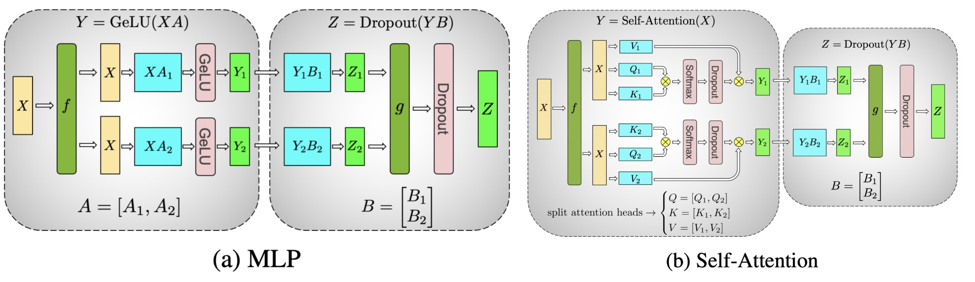
The following image from Megatron-LM paper comprises of everything very neatly. Take a look

Megatron LLM

Small Note

If you have n GPUs, the computational workload is divided by n per GPU. While this reduces computation time, the added communication overhead means the end-to-end latency won’t simply decrease by a factor of n. So if you load the same model on same class of GPU using varying tensor parallel degrees, aka 1,2,4 and 8, what I have noticed is that 1 GPU would perform better at latency than 2 GPUs. At 4 the tides generally tend to turn in favour of it over the 1 GPU case. This is due to the multi fold gains you get by distributing the load on even more GPUs. Do note that this is just an observation.

A rubric

Good, we’ve looked at the paradigms. But how does one decide when to use what? The key things to note should be

1. Avoid communication if possible.
2. Minimise communication if possible
   • Minimise communication over the network as much as possible

Any time you spend performing communication is time un-utilised for computation. Armed with this knowledge, I’d say

1. If your model/workload fits on one GPU, great, use data parallel and get gains with minimal to no losses.
2. If you have multiple GPUs in a single node, physically connected via say PCIe or NVLink or some super fast bandwidth, you can use tensor parallelism across those GPUs.
3. If your workload still isn’t satisfied, then you’d use pipeline parallelism across different nodes, which minimizes communication over the slower network links,

Conclusion

Today we’ve looked at how one can utilize multiple GPUs to their advantage especially in case of LLMs for inference. This is a very important in the modern day and age where models keep getting bigger and better increasing the demand for more and more memory at inference time more so thanks to reasoning and longer output lengths. That being said, we haven’t yet talked about how the communication is done between the GPUs. That is a different beast in itself. Also we haven’t yet touched upon the recent paradigms like Sequence Parallelism and Context Parallelism. Then comes parallelism strategies for training. We’d go over those too someday.

I’m hoping that I have made you, the reader, understand the parallelisms from a holistic perspective and the pros and cons of each. With that, I sign off for the day. Ta-ta.