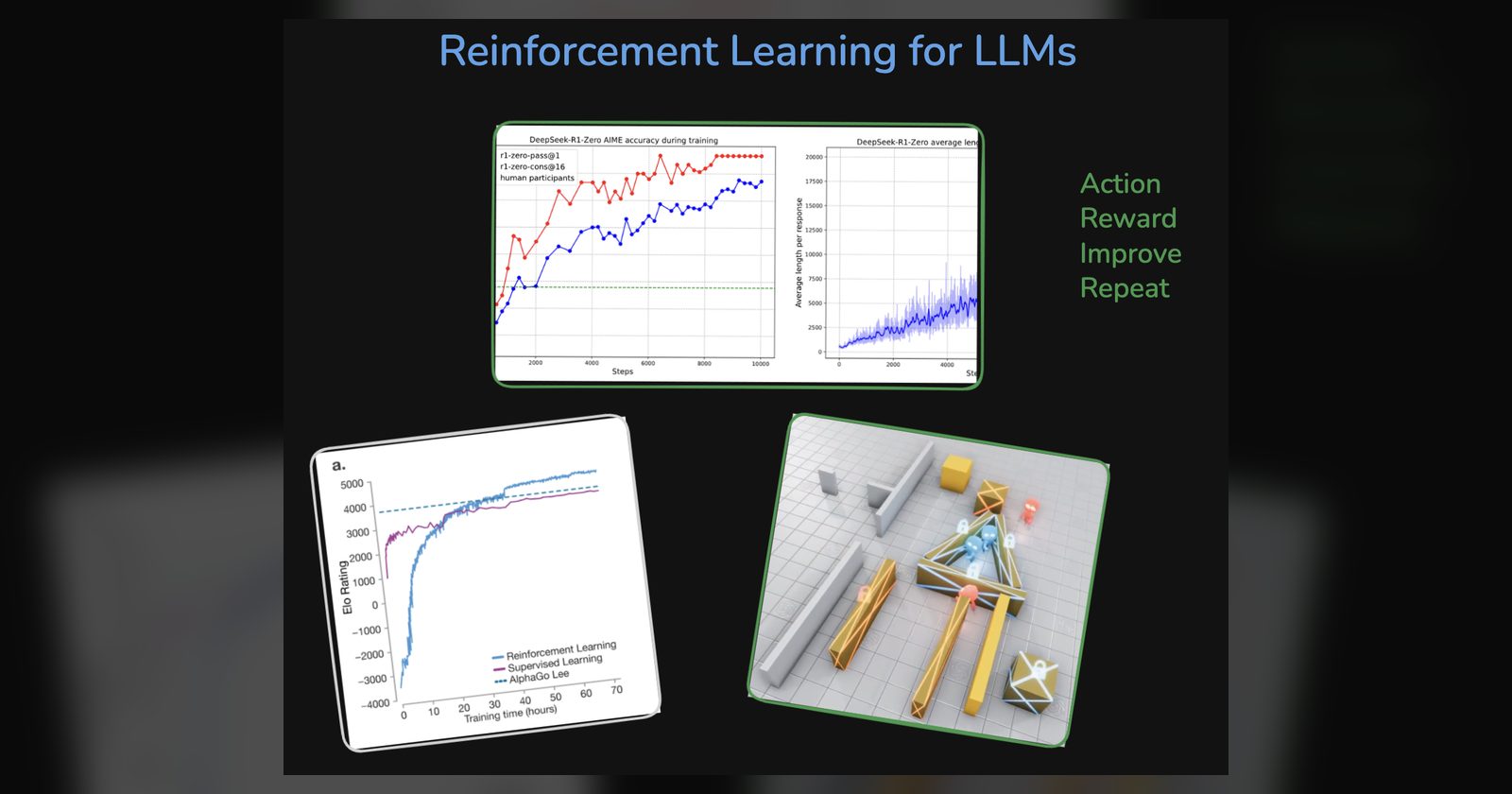
Reinforcement Learning for LLMs

Introduction

LLMs have come a long way in the last few years. We’ve gone from LLMs writing poems and short essays to seeing them solve hard math and coding problems. But they started as stochastic parrots, right? Regurgitating whatever they had read on the internet without any originality. How did we get them to make such a tremendous leap? Let’s find out. TLDR at the end.

Supervised Fine-Tuning

If you have a model that can understand internet-scale data and predict it reliably, then it is safe to assume that it has learned language and some basic knowledge of the world. Such a model only needs to be shown the ways of being a helpful assistant to be able to respond to our queries well. This is usually what SFT does. You teach the model to respond in certain formats, with certain traits. Typically the initial training on the internet corpus data is referred to as pretraining. The idea there is to let the model predict the next token, and that is what the loss optimizes for too. We call the loss cross-entropy loss.

\[\mathcal{L} = -\sum_{i=1}^{N} y_i \log(\hat{y}_i)\]

Here $y_i$ is the true label distribution and $\hat{y}_i$ is the predicted probability distribution.

So what’s the problem?

Well, the problem is, even with SFT, you’re still teaching the model by showing it example answers. I’d say this is like Imitation. And for everything you want to teach the model, you need explicit examples of what to do in each case. So data gathering is a big requirement as well. High-quality datasets at large scale are not easy to come by. Even then you might miss the niche cases that you didn’t have examples for, aka the tail of the distribution (whatever that means). For example, you might have a lot of Python code in the dataset but the model might still struggle to write good PyTorch code.

Reinforcement Learning

So to teach a kid to play chess, you can tell them to do move XYZ in situation ABC. But that is not enough for real games, because any deviation from studied theory makes them vulnerable. Sure, they might be able to pattern match and understand a few more scenarios than what you explicitly taught them. But beyond that, the scope for discovering novel and unique strategies is limited. The real learning and improvement happens when they play the game, do well or poorly, see the outcome, correct themselves, and repeat this loop. I’d go as far as to say that real learning happens at the boundaries of current knowledge and skill. The “play the game” part is taking “actions” in the “environment” of the chess board at different points of the game called “states”. The “do well or poorly” and “win/lose” part is the reward. This is pretty much how every reinforcement learning setup is structured.

• Agent: The learner (in our case, the LLM)
• Environment: Where your actions are applied. For LLMs, it is the task at hand (e.g. coding, math, gameplay, etc.). This can also be a collection of tasks and environments.
• State: The current position on the board (or the current context in the task)
• Action: The move made by the agent (or the response generated by the LLM)
• Reward: The outcome of the action (win/lose or the quality of the response)
• Policy: The strategy the agent uses to make decisions (or the LLM’s generation strategy)
• Value Function: The expected return of being in a particular state (or the expected quality from the current context). Only depends on the state. Denoted as $V(s)$
• Q-Function: The expected return of taking a particular action in a particular state (or the expected quality of a response given a context). Denoted as $Q(s, a)$

Let’s keep one LLM example in mind as we go. Say the prompt is a math problem, and the model samples a few answers:

• Completion A: fluent reasoning, but wrong final answer
• Completion B: correct final answer, but messy reasoning
• Completion C: correct final answer with clean reasoning

So what are the pieces here? The state is the prompt plus the tokens generated so far. The action can be the next token if you’re looking closely, or the whole completion if you’re zoomed out. The policy is the LLM sampling those tokens. The reward can come from a verifier, a human preference label, or a learned reward model. And the old SFT model often becomes the reference policy, basically the model we do not want to drift too far from.

Now that you have the task at hand set up, what exactly are we optimizing for? We want to let the model move towards policies that give higher returns. Because we are doing gradient descent, we would like to formulate a loss that can capture this exact thing.

\[\begin{aligned} \max_{\pi} \mathbb{J}(\pi) &= \mathbb{E}_{\pi}[R_t] \\ R_t &= r_t \\ R_t &= \sum_{t'=t}^{T} r_{t'} \\ R_t &= \sum_{t'=t}^{T} \gamma^{t'-t} r_{t'} \end{aligned}\]

One thing to notice here is that the return from time $t$ only accumulates rewards from $t$ onward. Why not include the rewards from the past too? Because we want to evaluate the value of being in the current state, or taking the current action, given what happens after it. Past rewards already happened and should not change how good this current decision is. If we included past rewards too, a bad action that follows a great opening could look better than a good recovery action that follows a bad opening. We do not want that.

How do we go about achieving this? You can either improve the policy to predict the best actions directly, or you can learn a Q-function that predicts the expected return for each state-action pair and then choose actions that maximize the Q value. Though this approach can lead to a small issue.

If a chess agent only sees near-optimal sequences of moves, it mostly reaches advantageous states and never learns how to handle disadvantageous positions or recover from them. It also might not be able to predict the best move in an amateur game.

One has to remember that any action/state you do not visit, you have no understanding about. So even if it is not the most optimal state, you might want to visit it every now and then. You can also explore variants like epsilon-greedy, where you randomly explore with a small probability instead of always choosing the max-reward action. The fine balance between exploration and exploitation is a key challenge in RL.

So what if we skip learning a separate Q-function and directly improve the policy itself? These are often called policy-gradient methods because we improve the policy directly with gradient ascent/descent. There need not be any explicit value function or Q-function here, though in practice many policy-gradient methods still use a value baseline to reduce variance.

Why Reinforcement Learning over Supervised Fine-Tuning?

Well, let’s look at history so that the RL fanboy in me doesn’t give you a biased opinion. DeepMind’s game-playing systems made this contrast very visible. Earlier AlphaGo systems used supervised learning to imitate expert human Go moves and then improved with reinforcement learning. AlphaGo Zero and AlphaZero pushed this further: they learned from self-play with no human game data, and AlphaZero reached superhuman play in chess, shogi, and Go. I rest my case.

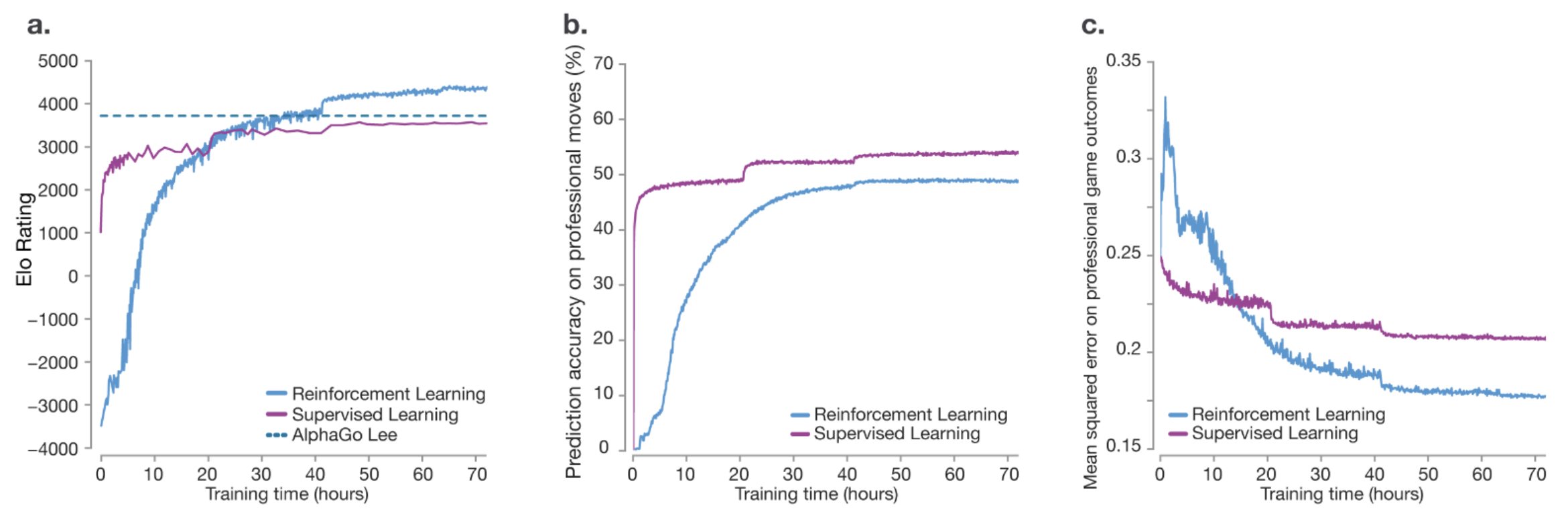RL vs SFT on Go

Before we jump into the math, there is one annoying bit. We cannot directly backpropagate through the sentence “this sampled answer was good”. The reward comes after the model has sampled text. So how do we update the model if the reward is not a differentiable function of the tokens? REINFORCE is the trick that lets us increase or decrease the probability of sampled text using only its log probability and the reward it received.

REINFORCE

This is pretty much the foundation of many modern policy-gradient algorithms and one among the earliest policy-gradient methods. In the simplest form, the formulation is to maximize the expected reward. So the objective is to

\[\max_{\pi} \mathbb{J}(\pi) = \mathbb{E}_{x \in D,\, y \sim \pi_{\theta}(\cdot|x)}[R(x,y)]\]

But our optimizers usually minimize losses, right? So we formulate this as a minimization problem of the negative of the above.

\[\min_{\pi} -\mathbb{J}(\pi) = -\mathbb{E}_{x \in D,\, y \sim \pi_{\theta}(\cdot|x)}[R(x,y)]\]

But for that to happen, we need to be able to define what the gradient is. The reward is given by the environment and y is just a sampled rollout from the policy. You might think, “why not take the derivative of the expectation?” You are right in thinking that. Let’s look at the math first.

\[\begin{aligned} \nabla_{\theta} \mathbb{J}(\pi_{\theta}) &= \nabla_{\theta} \mathbb{E}_{x \in D,\, y \sim \pi_{\theta}(\cdot|x)}[R(x,y)] \\ &= \nabla_{\theta} \sum_{x \in D}\sum_y \pi_{\theta}(y | x) R(x,y) \\ &= \sum_{x \in D}\sum_y \nabla_{\theta}\pi_{\theta}(y | x) R(x,y) \end{aligned}\]

The problem here is if we choose to take the derivative of the probability distribution, we end up with a complex expression that is hard to compute. We would also lose the ability to represent this as an expectation. The moment we formulate it as expectation, we can use the samples to estimate the gradient. So the question becomes, how do we have the gradient operation while also having a $\mathbb{P}(y \mid x)$ in the expression?

The log trick

Remember $\frac{d}{dx} \log x = \frac{1}{x}$? Because the derivative of log gives us the inverse of the original function, we can use this to our advantage. So we have

\[\nabla \log \pi_{\theta}(y|x) = \frac{1}{\pi_{\theta}(y|x)} \nabla \pi_{\theta}(y|x)\]

which means

\[\nabla \pi_{\theta}(y|x) = \pi_{\theta}(y|x) \nabla \log \pi_{\theta}(y|x)\]

Substituting this back into our original expression, we get

\[\nabla_{\theta} \mathbb{J}(\pi_{\theta}) = \sum_{x \in D}\sum_y \pi_{\theta}(y | x) \nabla \log \pi_{\theta}(y | x) R(x,y)\]

Now we have a probability term inside, multiplied by a function/expression and a summation wrapping the entire thing. That is the classic Expectation formulation, almost akin to what we started with. So we can write this as

\[\nabla_{\theta} \mathbb{J}(\pi_{\theta}) = \mathbb{E}_{x \in D,\, y \sim \pi_{\theta}(\cdot|x)} \left[\nabla \log \pi_{\theta}(y|x) R(x,y)\right]\]

All great. But is raw reward enough? If the agent is already in a good state (almost winning a chess game), many actions might lead to positive reward. In our math-prompt example, an easy prompt might make all three completions look decent, even if one is better than the others. Without a baseline, all sampled actions can get reinforced just because the state was already good. This is noisy and not ideal. So what do we compare the reward against? We subtract a baseline from the reward. This baseline is usually a proxy for how good the state is before choosing the action. This helps reduce the variance of the gradient estimate. The formulation now becomes… It is very important that the baseline does not depend on the sampled action $y$. It can depend on $x$; if it is learned, its parameters are usually handled separately from the policy-gradient term.

\[\nabla_{\theta} \mathbb{J}(\pi_{\theta}) = \mathbb{E}_{x \in D,\, y \sim \pi_{\theta}(\cdot|x)} \left[ \nabla \log \pi_{\theta}(y|x)(R(x,y) - b(x)) \right]\]

where $b(x)$ is the baseline.

PPO

This is one of the workhorse reinforcement learning algorithms used in RLHF. It is pretty much some more mathematical adjustments on top of REINFORCE. The baseline-subtracted reward is typically called the advantage here. In the initial days of LLMs, especially around GPT-3 and InstructGPT, there was a need for a way to train models to be helpful, truthful, harmless, etc. All the qualities that are easier to judge and harder to quantify mathematically. So one way was to use reinforcement learning where helpful and correct responses would get higher rewards. But unlike pretraining or supervised fine-tuning, this involves generation. Generating 1000 new tokens takes 1000 autoregressive decoding steps, whereas in pretraining/SFT a 1000-token sample can be trained with a single teacher-forced forward pass.

Before the equations, why does PPO need all these extra terms? Here’s the quick cheat sheet:

Problem	PPO ingredient
Rollouts are expensive	Reuse rollout batches for multiple updates
Reusing old rollouts creates policy mismatch	Importance-sampling ratio
Updates can become too large	Clipped surrogate objective
Model can drift away from SFT behavior	KL penalty against the reference model
Rewards are noisy	Critic/value baseline

So to make it more efficient, can we reuse the same rollout batch for multiple updates? We can, but we have to make sure that the policy (weights) that generated the rollout is not too far off from the current policy (weights) that we are doing gradient updates on. For the first step, this is exactly the same policy (ignoring trainer-inference mismatch, which is a separate problem). But if we want to do, say, 4 steps, the policy would have changed by the 2nd step and the mismatch needs to be mathematically addressed.

In case of mismatch, the expectation (which is over generations $y$) is over $\theta_{old}$, but the logprobs and gradient are computed using the current $\theta$.

The importance sampling correction

Consider a probability distribution P for which you want to calculate the expectation over. But you unfortunately do not have access to samples from P. Instead you can sample from another distribution Q over the same input space. How would one calculate that?

\[\begin{aligned} \mathbb{E}_P[f(x)] &= \sum_x P(x) f(x) \\ &= \sum_x \frac{P(x)}{Q(x)} Q(x) f(x) \\ &= \mathbb{E}_Q\left[\frac{P(x)}{Q(x)} f(x)\right] \end{aligned}\]

So here we converted an expectation over P to an expectation over Q by reweighting the samples with the ratio $\frac{P(x)}{Q(x)}$. This is exactly what we’re about to do to the PPO case as well. Q is the fixed distribution that generated the rollouts. P is the distribution we’re optimizing and gradient updating on. We’re going to explain what $A^\pi(x, y)$ is later.

\[\begin{aligned} \nabla \mathbb{J}(\theta) &= \mathbb{E}_{x \sim \mathcal{D},\, y \sim \pi_\theta(\cdot|x)} \left[\nabla \log \pi_\theta(y|x) A^\pi(x,y)\right] \\ &= \mathbb{E}_{x \sim \mathcal{D},\, y \sim \pi_{\theta_{old}}(\cdot|x)} \left[ \frac{\pi_\theta(y|x)}{\pi_{\theta_{old}}(y|x)} \nabla \log \pi_\theta(y|x) A^\pi(x,y) \right] \end{aligned}\]

The trust region

One other thing when it comes to RL is, unlike SFT which is often forgiving of setup choices, RL is very finicky. Small changes in the setup can cause drastic differences. The range is as wide as learning vs collapsing. So we need to be careful. There can be rogue data samples or rollouts which spoil the training process. Also we need to make sure noise in the environment, reward, or rollouts does not mess it up. So we want to make sure the updates are “capped” so that consistent changes in a similar direction will result in learning, but random changes and noise do not have too much impact. This is where “trust region” comes in. Because the update has an importance-sampling factor, which is a useful measure of how far the new policy is from the old policy on sampled actions, we try to clamp it to achieve that.

\[\begin{aligned} A^{\pi}(x,y) &= R(x,y) - b(x) \\ \rho(\theta) &= \frac{\pi_\theta(y|x)}{\pi_{\theta_{old}}(y|x)} \end{aligned}\] \[\mathbb{J}(\theta) = \mathbb{E}_{x \sim \mathcal{D},\, y \sim \pi_{\theta_{old}}(\cdot|x)} \left[ \min\left( \rho(\theta) A^\pi(x,y), \operatorname{clip}(\rho(\theta), 1-\epsilon, 1+\epsilon) A^\pi(x,y) \right) \right]\]

Note that the advantage can be both negative and positive for a given batch. So we want to look into how the trust-region clipping works in both cases. Assuming the usual $\epsilon = 0.2$, we have…

The clipping handles the two signs of advantage differently:

Advantage	Not clipped	Clipped
Positive advantage good answer reinforce	$\rho_t(\theta)\hat{A}_t$ answer is good not over-updated yet gradient can still increase probability	$(1+\epsilon)\hat{A}_t$ answer is already sufficiently more likely gradient is stopped
Negative advantage bad answer discourage	$\rho_t(\theta)\hat{A}_t$ answer is bad not over-updated yet gradient can still decrease probability	$(1-\epsilon)\hat{A}_t$ answer is already sufficiently less likely gradient is stopped

epsilon = 0.20

The plot shows $\min(\rho A, \operatorname{clip}(\rho, 1-\epsilon, 1+\epsilon)A)$ for $A=1$ and $A=-1$. The shaded band is the trust region.

A useful mental model is to view the clipping behavior as a mask on the policy-gradient contribution:

\[M(\hat{A}_t,\rho_t,\epsilon) = \begin{cases} 0, & (\hat{A}_t > 0 \land \rho_t > 1+\epsilon) \lor (\hat{A}_t < 0 \land \rho_t < 1-\epsilon) \\ 1, & \text{otherwise} \end{cases}\]

So the policy-gradient contribution can be viewed as:

\[\mathbb{J}(\theta) = \mathbb{E}_{x \sim \mathcal{D},\, y \sim \pi_{\theta_{old}}(\cdot|x)} \left[ M(\hat{A}_t,\rho_t,\epsilon)\rho(\theta)A^\pi(x,y) \right]\]

Do note that this is only a mental model for where the gradient stops; the actual PPO objective is still the clipped surrogate shown above. When the mask is zero, the policy-gradient contribution from that clipped ratio is zero. So for learning to happen, we need samples to be just hard enough that improvement is reachable for the model, but not so far away that the update gets clipped all the time.

The KL divergence penalty

All is great so far. We formulated REINFORCE with baseline subtraction for reduced variance, added importance sampling to relieve rollout pressure, and added trust-region clipping to keep updates from getting too big. But do we want the model to freely move away from the SFT model? Not really. The SFT model we created already has a lot of capabilities and preferences baked into it. We do not want to stray too far from it. So we add a KL divergence penalty with respect to the same SFT model, often called the reference model, so that we don’t drift too far off from it either.

So the final objective becomes:

\[\begin{aligned} \mathbb{J}(\theta) = \mathbb{E}_{x \sim \mathcal{D},\, y \sim \pi_{\theta_{old}}(\cdot|x)} \Big[ &\min\left( \rho(\theta) A^\pi(x,y), \operatorname{clip}(\rho(\theta), 1-\epsilon, 1+\epsilon) A^\pi(x,y) \right) - \beta \,\mathrm{KL}\left( \pi_\theta(\cdot|x) \,\|\, \pi_{\text{ref}}(\cdot|x) \right) \Big] \end{aligned}\]

where $\beta$ is the KL divergence penalty coefficient, typically small enough that KL divergence doesn’t overpower the environment reward but large enough to prevent the policy from drifting too far. So even while maxing out on math and code, your model doesn’t forget the language, knowledge, and chat-assistant capabilities it had before.

The LLM Setup

So how does all this map to LLMs in practice? One early famous setup was InstructGPT, where the task was to make the model follow instructions while being helpful, truthful, and harmless. The LLM is the actor, the generations are actions, and the reward model turns human preference feedback into a scalar reward.

But now the question becomes how do you even get rewards here? Well, one way is to let humans score every completion the model generates, but this is not scalable. One simply can’t sit and rate millions of completions that the model generates throughout the training process.

The reward model

So what is our next best bet here? Well, if models are good enough to generate text, we can train a similar model to judge which outputs humans prefer. The general trend in deep learning is that verifying something is often easier than generating it. Off topic, but this is why GANs were the early pioneers of image generation. I’ll let you think about why this is being mentioned here :)

Typically the LLM architecture looks as follows:

Generation: tokens -> embeddings -> decoder layers -->
            lm_head: nn.Linear(model_dim, vocab_size) -> sampled token

For a reward model we have

Reward model: tokens -> embeddings -> decoder layers -->
              reward_head: nn.Linear(model_dim, 1) -> scalar reward

Do we need to invent a completely new architecture for this? Not really. Most of the backbone can stay the same if we were to train a reward model. The only thing we need to change is that, instead of predicting probabilities over the token space (using lm_head), we need to predict a scalar reward value.

And once we have preference data, we can train this reward model, which is often initialized from the SFT model with lm_head swapped out for reward_head. In our math example, if the actor model generates completions A/B/C, the reward model is trained to score which completion humans would prefer. It should learn that a correct and clean completion is better than a fluent but wrong one.

But scoring completions might lead to ambiguity. One person’s preference on one of the factors might overpower another person’s preference on a different factor. What else can be easier and more consistent? Well, if you can’t rate something, you can at least compare it against something else and pick what is better. But then how do we turn “A is better than B” into a smooth training objective? Given the noisy nature of human preferences and the discontinuity in the preference function (it is either a win=1 or a loss=0, no in-between), we turn to a probabilistic model called Bradley-Terry, which models the probability that one item is preferred over another.

\[P(A > B) = \sigma(R_W - R_L) = \sigma (r_{\phi}(x, y_w) - r_{\phi}(x, y_l))\]

where $\sigma$ is the sigmoid function and $R_W$ and $R_L$ are the rewards for the winning and losing items respectively. The probability of winning is higher when the reward difference is higher. Sigmoid maps the reward difference into the $(0,1)$ range. The $r_{\phi}$ term represents the reward the model predicts.

The optimization criteria for the reward model therefore looks like

\[\mathcal{L}_{reward} = -\log P(y_w > y_l | x) = -\log \sigma(r_{\phi}(x, y_w) - r_{\phi}(x, y_l))\]

If $r_w - r_l$ is large positive: sigmoid ≈ 1, $-\log(\sigma) ≈ 0$. We’re good

If $r_w - r_l = 0$: sigmoid = 0.5, loss = $-\log(0.5) ≈ 0.693$

If $r_w - r_l$ is negative: sigmoid < 0.5, loss is large

Do note that we score the entire completion. The reward is for the entire rollout and not per token. So just like when trying to predict the next token, we forward pass the entire hidden-state tensor of shape (seq_len, hidden_dim) and use the final token representation. For generation, that final hidden state is multiplied by lm_head; for reward modeling, it is multiplied by reward_head to get the sequence reward. In a causal decoder, the final token can attend to the previous tokens, so it can serve as a summary position for the sequence. Read my previous blog for an in-depth understanding of the same.

Caution is advised

But what happens if the reward or environment has a tiny loophole? When OpenAI trained agents to play hide-and-seek in an environment with some movable objects, they found some cool emergent behavior. This is also a good reminder that reward design and environment design matter a lot in RL. Small loopholes can become big learning signals.

1. Hiders construct shelters

2. Seekers learn box surfing. Here the agent is exploiting a loophole in the environment

3. Hiders lock objects (in game ability, intentional)

The value/critic model

Great, we tackled one problem of reward assignment. We also need to think about the “baseline” calculation given a prompt, right? After all, that is what stabilizes the training process. In the chess example, the baseline would be the evaluation of the given position. In the math-prompt example, it is closer to asking, “How much reward should we expect from this prompt before seeing this particular sampled completion?” Neither scoring the answer, nor predicting the answer. Just evaluating the current state.

Well, you know the script by now. Can humans provide this baseline for every prompt and every partial completion? Obviously not. Just like reward model, when we can’t scalably do it with humans, we offload it to models. Welcome to yet another model :). This one is again pretty similar to the reward model.

Critic model: tokens -> embeddings -> decoder layers -> 
              value_head (model_dim -> 1) -> value per token

The tried and tested method

Now the question is whether you want KL divergence to be just an auxiliary/helper term or a primary part of the objective. Should the critic predict only the external reward, or the reward after KL has already been accounted for? In PPO-style RLHF, it is common to include the KL penalty in the reward itself, rather than as a last step to mend things. So we let the value model predict the discounted/aggregated future reward, which can also include the KL divergence penalty per token.

So the optimization criteria becomes

\[\begin{aligned} \mathcal{L}_{critic} &= \frac{1}{2}\left(\mathcal{R} - V_{\theta}(s)\right)^2 \\ \mathcal{R}_{MC} &= r_t + \gamma r_{t+1} + \gamma^2 r_{t+2} + \dots \\ \mathcal{R}_{TD} &= r_t + \gamma V_{\theta}(s_{t+1}) \end{aligned}\]

The idea is that the value of a state can be estimated in many ways. It can be Monte Carlo, where we depend on rollout rewards, or TD(k), where we use the next k states’ values to estimate the value of the current state.

Generalized Advantage Estimation (GAE)

In PPO we use something called Generalized Advantage Estimation (GAE), which is a combination of TD and Monte Carlo-style estimates. The idea is Monte Carlo is less biased but noisy because it depends on full rollouts. TD is more stable but biased because it bootstraps from a value estimate. GAE combines both by using an exponentially weighted sum of TD residuals.

\[\begin{aligned} \mathcal{R} &= A^{GAE}_t + V_{\text{old}}(s_t) \\ A^{GAE}_t &= \sum_{l=0}^{T-t}(\gamma\lambda)^l \delta_{t+l} \\ \delta_t &= r_t + \gamma V_{\text{old}}(s_{t+1}) - V_{\text{old}}(s_t) \end{aligned}\]

Notice the “old” here? These are the value predictions from the model snapshot used around rollout collection, not the value model after several PPO update steps. It is the same stale-data issue as the $\pi_{old}$ from the beginning of our PPO discussion.

Because this value prediction is a per-token thing, can we just take the last hidden state like the reward model? Not really. We take the entire (seq_len, hidden_dim) sized tensor and pass it through a linear layer to get a scalar value for each token. One pass per sequence, akin to pretraining of LLMs.

DPO

PPO is great, but one needs to maintain a reward model and a value model. Both need their own training. If the model is so smart that it can predict the reward and also the value of a state, why not let it do the preference optimization implicitly and skip the extra models altogether? We anyway have pairwise preference data. No separate reward model, no value model. Sounds good, right? That is exactly what DPO does. The paper itself was titled “Direct Preference Optimization: Your Language Model is Secretly a Reward Model”. But for that we need to make some small sacrifices. We drop the advantage estimate and clipping for an easier and simpler formulation.

In our running example, DPO would take pairs like “Completion C is preferred over Completion A” and directly push the policy toward the preferred completion relative to the reference model. The nice part? No online rollout loop is needed during this preference-tuning step.

Let’s start with the basic KL-regularized objective akin to REINFORCE:

\[\begin{aligned} \mathcal{L} &= \mathbb{E}\left[ r(x,y) - \beta \log \frac{\pi(y|x)}{\pi_{ref}(y|x)} \right] \\ \mathrm{KL}(p \| q) &= \mathbb{E}_p\left[\log(p/q)\right] \\ \pi^*(y|x) &\propto \pi_{ref}(y|x)\exp\left(\frac{1}{\beta}r(x,y)\right) \end{aligned}\]

The derivation for those interested (click to expand)

\[\begin{aligned} \mathcal{L} &= \mathbb{E}\left[ r(x,y) - \beta \log \frac{\pi(y|x)}{\pi_{ref}(y|x)} \right] \\ &= \sum_{x,y}\pi(x,y) \left[ r(x,y) - \beta \log \frac{\pi(y|x)}{\pi_{ref}(y|x)} \right] \end{aligned}\]

The constraint is:

\[\sum_y \pi(y|x) = 1\]

So the Lagrangian is:

\[\mathcal{L}_{\text{lag}} = \sum_{x,y}\pi(x,y) \left[ r(x,y) - \beta \log \frac{\pi(y|x)}{\pi_{ref}(y|x)} \right] - \lambda\left(\sum_y \pi(y|x) - 1\right)\]

Using $\frac{d}{dp}p\log p = \log p + 1$, we get:

\[\begin{aligned} \frac{d}{d\pi}\mathcal{L}_{\text{lag}} &= r(x,y) - \beta \log \frac{\pi(y|x)}{\pi_{ref}(y|x)} - \beta - \lambda \\ &= 0 \\ \pi(y|x) &\propto \pi_{ref}(y|x) \exp\left(\frac{r(x,y)-\beta-\lambda}{\beta}\right) \end{aligned}\]

\[\begin{aligned} \pi^*(y|x) &\propto \pi_{ref}(y|x)\exp\left(\frac{1}{\beta}r(x,y)\right) \\ r(x,y) &= \beta \log \frac{\pi^*(y|x)}{\pi_{ref}(y|x)} + C \\ r(x,y_w) - r(x,y_l) &= \beta \log \frac{\pi^*(y_w|x)}{\pi_{ref}(y_w|x)} - \beta \log \frac{\pi^*(y_l|x)}{\pi_{ref}(y_l|x)} \end{aligned}\]

What a clean, simple, and minimal formula we have arrived at. This will also change our objective function.

\[\begin{aligned} \mathcal{L}_{\text{DPO}} &= -\log \sigma\left(r(x,y_w)-r(x,y_l)\right) \\ &= -\log \sigma\left( \beta \log \frac{\pi_\theta(y_w|x)}{\pi_{ref}(y_w|x)} - \beta \log \frac{\pi_\theta(y_l|x)}{\pi_{ref}(y_l|x)} \right) \end{aligned}\]

No need for a separate reward model, no critic model, and no online rollout loop during fine-tuning. A lot of compute and time saved. This has been one of the go-to methods for preference tuning over the last few years.

GRPO

OK last one, I promise :). If you followed the AI and LLM world closely or from afar, you’d have heard DeepSeek-V3 and DeepSeek-R1 making massive waves. Some American AI-linked stocks fell sharply during that phase in early 2025. Though R1 was the model that made the biggest mainstream headlines, the seeds for this recipe were sown earlier in the DeepSeekMath paper. What is the seed, you ask? The thing that helped models chase the IMO dream and also go on to become some of the best coding models in the world. This technique is called Group Relative Policy Optimization (GRPO).

So when you have pre-annotated preference data, PPO/DPO work well. But what about math and code? Do we really need humans to judge every completion there? Verification is much easier than generation. That pretty much looks like a task made in heaven for RL. So the reward part of the setup is easy. For math, see if the answer matches the expected answer and score it accordingly. For code, run it on a test suite. You get the idea. Let’s call these reward functions.

But now what about value estimation? Do we really need a separate critic if we already sampled multiple completions for the same prompt? Well, this is where GRPO really shines. Instead of trying to estimate the value of each individual completion with a critic, GRPO looks at groups of completions for a given prompt and compares them relative to each other. If the group itself gives you a decent baseline, you can skip the learned value model.

Why does this make sense? For an easy prompt, all the completions would get good reward from the functions, but when you take relative reward, that will die down to zero. There isn’t much to learn when all the completions are equally good anyway. On the other hand, for a hard prompt, some completions will be much better than others and the relative reward will be high. This is where the learning happens. Mathematically:

\[A_{\text{GRPO}} = \frac{ r(x,y) - \mathbb{E}_{y' \sim \pi_{\theta}}[r(x,y')] }{ \sigma_{y' \sim \pi_{\theta}}[r(x,y')] }\]

The original formulation normalized the advantage by the group standard deviation to keep the scale controlled. When the group std is small, this division also amplifies small reward differences. Later work such as Dr. GRPO argued that parts of the GRPO objective can introduce optimization bias, especially around response length, and proposed a modified objective. The point is, normalization and length scaling need care, because tiny objective details can change the training dynamics a lot.

\[\mathcal{L}_{\mathrm{GRPO}}(\theta) = -\mathbb{E}_{q,\{o_i\}_{i=1}^{G}} \left[ \frac{1}{G}\sum_{i=1}^{G} \frac{1}{|o_i|} \sum_{t=1}^{|o_i|} \ell_{i,t}(\theta) \right]\]

where the per-token objective is:

\[\ell_{i,t}(\theta) = \min\left( \rho_{i,t}(\theta)\hat{A}_i,\, \operatorname{clip}\left(\rho_{i,t}(\theta),1-\epsilon,1+\epsilon\right)\hat{A}_i \right) - \beta D_{\mathrm{KL}}\left(\pi_\theta \,\|\, \pi_{\mathrm{ref}}\right)\]

So the DeepSeek team used GRPO-style RL to train models on math and code and saw behaviors like self-correction and self-critiquing, including the so-called “aha” moment in DeepSeek-R1. There were two notable variants: DeepSeek-R1-Zero, trained directly with RL from the base model, and DeepSeek-R1, which used cold-start reasoning data before RL. The latter recipe is more common now. Do note that response length going up can be both a sign of the model thinking longer and a sign of biased optimization criteria. In the loss function above, the per-completion term is divided by the length of the completion. This means for equal advantage, longer completions have lower loss than shorter ones thus biasing the training towards longer sequences. Objective choices like this can affect length behavior, which is why caution is advised when doing RL.

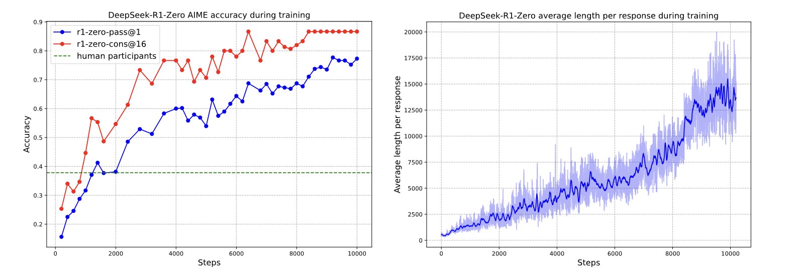Reward achieved by DeepSeek-R1

Another advantage GRPO gives in math/code settings is that the reward functions can be deterministic and hence the rewards are very verifiable. Why is that a big deal? You’re not at the mercy of a learned reward model to give you the right rewards and then train the downstream task. People often call this Reinforcement Learning from Verifiable Rewards or RLVR.

But what if the reward is not verifiable, like helpfulness or harmlessness? You can fall back to training a model to predict the rewards, but the idea is you at least eliminate a critic here. That alone amounts to a decent amount of memory savings. But at that point you might want to compare it with DPO, which doesn’t need a separate reward model during policy training.

Putting it side by side

Method	Needs online rollouts?	Needs reward model?	Needs critic/value model?	Best fit
PPO	Yes	Often	Yes	RLHF with learned rewards
DPO	No	No	No	Pairwise preference data
GRPO	Yes	No for RLVR	No	Math, code, and verifiable rewards

TLDR

• RL can go beyond SFT when the reward is clear. Learning over imitation.
• REINFORCE is the backbone for policy-gradient methods.
• Baseline subtraction reduces variance. KL divergence with respect to the SFT/reference model acts as an anchor. Trust-region clipping improves stability.
• PPO is a major RLHF algorithm for LLMs, but it commonly uses an actor, reward model, value model, and reference model.
• DPO makes the reward implicit. Only chosen-rejected preference pairs are needed. No separate reward or critic model during policy training.
• GRPO uses group statistics as the baseline. No critic is needed. Verifiable rewards are the big deal here.

Final thoughts

Reinforcement learning has been the go-to for surpassing human-level performance on games, and it is now a major ingredient in tasks like math and coding. It comes in different flavors and you’re free to pick whatever you like. But the key is to test the waters before diving deep in. Today we mostly looked at the math and intuition behind the formulations. In the future we’ll go over the systems side of it. Given the insane amount of memory required for maintaining all those copies and the different components at play like trainer, inference engine etc, it becomes a very big task to manage the systems and make sure that they are in sync. It’s going to be another exciting blog, so stay tuned. Until then, happy brainstorming!

References

• AlphaZero: Mastering Chess and Shogi by Self-Play with a General Reinforcement Learning Algorithm
• OpenAI: Emergent Tool Use from Multi-Agent Interaction
• Proximal Policy Optimization Algorithms
• Hugging Face Deep RL Course: Visualize the Clipped Surrogate Objective Function
• Training Language Models to Follow Instructions with Human Feedback
• Direct Preference Optimization: Your Language Model is Secretly a Reward Model
• DeepSeekMath: Pushing the Limits of Mathematical Reasoning in Open Language Models
• DeepSeek-R1: Incentivizing Reasoning Capability in LLMs via Reinforcement Learning
• Understanding R1-Zero-Like Training: A Critical Perspective
• State of RL for Reasoning LLMs