Systems for LLM RL

Introduction

We have previously delved into RL for LLMs where we talked about how the math is formulated, how we go from a chatbot-style model to one that thinks, reasons, solves math, and writes code at superhuman levels of performance. But all this doesn’t come for free. Today we look at the systems challenges for the same and also look at how people go about solving them.

A brief about RL for LLMs

If you haven’t read the previous post yet, I strongly recommend reading that first. But if you don’t want to, here’s a short summary.

TLDR: RL for LLMs

• RL can go beyond SFT when the reward is clear. Learning over imitation.
• REINFORCE is the backbone for policy-gradient methods.
• Baseline subtraction reduces variance. KL divergence with respect to the SFT/reference model acts as an anchor. Trust-region clipping improves stability.
• PPO is a major RLHF algorithm for LLMs, but it commonly uses an actor, reward model, value model, and reference model.
• DPO makes the reward implicit. Only chosen-rejected preference pairs are needed. No separate reward or critic model during policy training.
• GRPO uses group statistics as the baseline. No critic is needed. Verifiable rewards are the big deal here.

Method	Online rollouts / on-policy updates?	Reward model?	Critic / value model?	Best fit
PPO	~Yes	Often	Yes	RLHF with learned rewards
DPO	No	No	No	Pairwise preference data
GRPO	~Yes	No for RLVR	No	Math, code, verifiable rewards

The systems requirements

Most of the RL algorithms need samples generated from the model we’re optimising for. When you generate samples from the same policy/model that you’re optimising, it is called on-policy learning. On the other hand, if you generate samples from another policy, perhaps a different model or a model that is a few optimisation steps behind (like we discussed in PPO), this is called off-policy learning.

In the case of PPO and GRPO, because we generate samples from the model that is being optimized, they come under online reinforcement learning. But we do accept some degree of off-policy drift. In the case of a chess-playing agent, on-policy learning is where it generates the moves and tries to learn from them. Off-policy is basically watching someone else generate the moves and learning from them. PPO is somewhere in between, where you generate one sequence of moves and try to do multiple gradient updates on it, taking advantage of importance sampling.

As we previously discussed, unlike SFT, the generation phase involves multiple forward passes through the model. So it is safe to assume that a large fraction of each on-policy RL training step, often the majority at higher sequence lengths, goes towards rollout generation. So it is very important to optimize inference both from a speed standpoint and from a memory usage standpoint. Many frameworks rely on hyper-optimized inference engines like vLLM or SGLang and delegate rollout generation to them.

Though this does come with some benefits, it also comes with its own challenges.

• Inference server, whether colocated (on same GPU(s)) or running standalone (on different GPUs), takes up GPU memory.
• Trainer, the model we’re optimising, also takes up GPU memory
• Reference model needs its own share
• In cases like PPO, you also need a value model and its own optimisation
• Once you introduce a separate process to generate rollouts (like vLLM), you need to make sure it stays up to date with the weights.

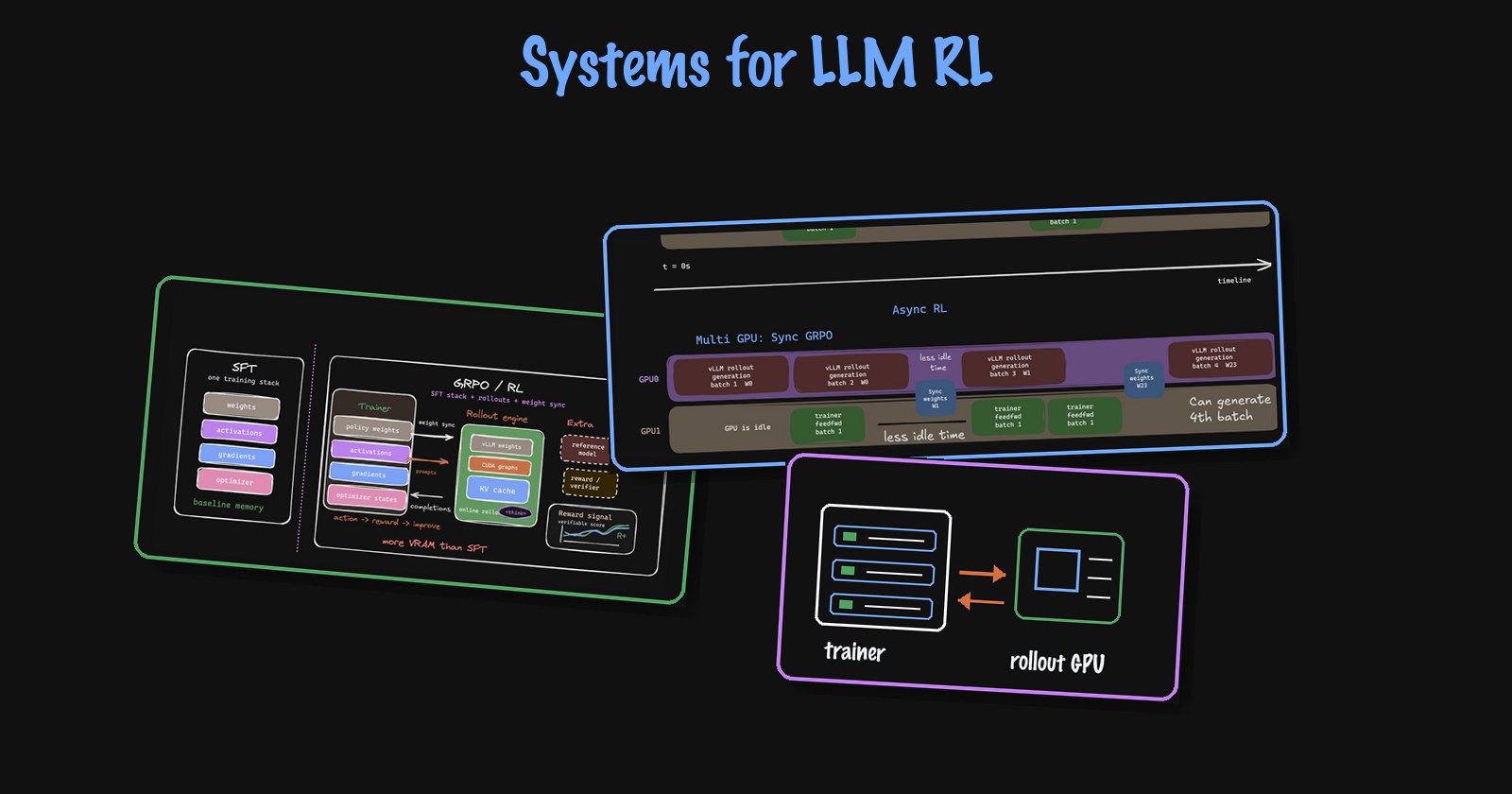
At a high level, this is why online RL feels much heavier than SFT. SFT mostly keeps one training stack alive: model weights, activations, gradients, and optimizer state. GRPO/RL adds a rollout engine that must generate thinking traces/completions, maintain inference-time state like KV cache, score samples with rewards/verifiers, and then sync updated trainer weights back into the inference engine. So the problem is not just “more memory”; it is also coordinating two systems that both need a fresh enough copy of the same policy.

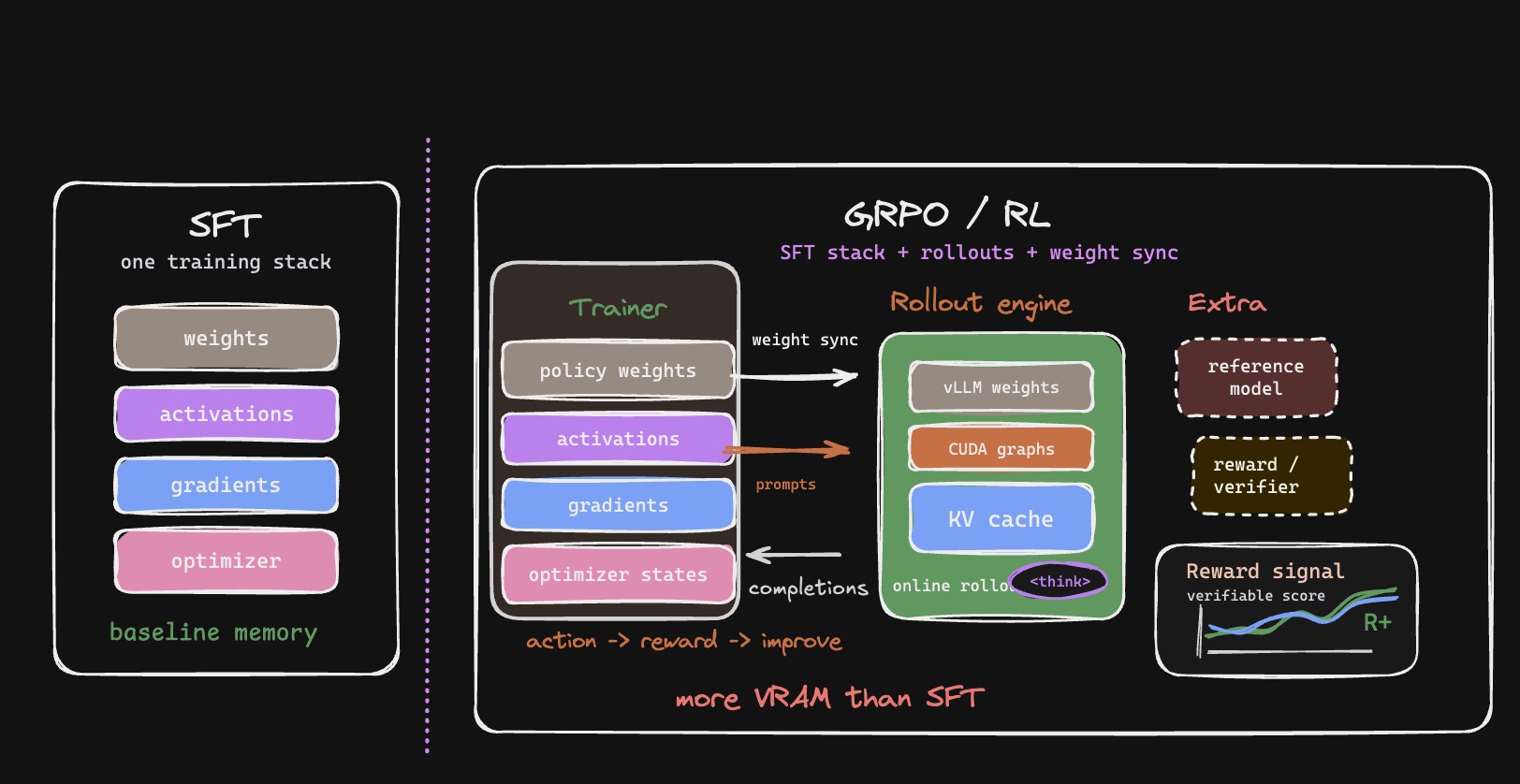Compared with SFT, online RL adds rollout memory and a weight-sync path between trainer and inference.

Let’s go through this methodically and try to analyse the memory requirement of the same.

VRAM is gone…

For training these are the biggest components that consume VRAM. Assuming that the model is n billion params

• Weights: n billion = 2n GB in BF16
• Gradients: n billion = 2n GB in BF16
• Optimizer states: 2 per param for Adam: 2 moving averages (moments). 2n billion = 8n GB in FP32 (typically higher precision)
• Master weights: n billion = 4n GB, sometimes stored to perform accumulation with the optimiser.
• Activations: Assuming you do activation checkpointing and use techniques like flash attention, this is often smaller than optimizer state at moderate sequence lengths, but it can still become significant for long-context RL.

Do note that you can also offload optimizer states and gradients to CPU as well. But any offload is bound to cause slowdowns. For activations, you offload some, persist some, recalculate some, etc.

For inference server: Assuming that you have l layers, $n_h$ query heads, $n_{kv}$ key-value heads each of dimension hs, hidden size h, and MLP dimension i for sequence length s and batch size b…

• Weights: n billion = 2n GB in BF16
• Transient activations/workspace: this depends a lot on prefill vs decode, CUDA graphs, batch token count, and the kernels being used. A rough activation-style estimate is $4 \times s \times b \times ((n_h + n_{kv}) \times hs + 3 \times i )$ bytes, but engines like vLLM mostly plan around weights and the profiled/preallocated KV cache budget.
• KVCache: Each layer stores key and value vectors for each KV head: $4 \times l \times b \times s \times (n_{kv} \times hs)$ bytes in BF16.

So let’s take the example of Qwen3-8B, which has 36 layers, 32 attention heads, 8 KV heads, a hidden size of 4096, and an MLP dimension of 12288. This is how the memory requirement looks like:

Qwen3-8B rollout memory sketch

Change the rollout shape and watch where the inference-side VRAM goes.

0.0 GiB

total

Sequence length

4096

Batch size

16

Weight dtype

BF16 / FP16

BF16 / FP16 weights FP32 weights

Weights

0.0 GiB

Activations

0.0 GiB

KV cache

0.0 GiB

Model shape controls

Layers

Hidden size

Query heads

KV heads

MLP size

Approximate inference/rollout memory only. This excludes framework overhead, fragmentation, CUDA workspaces, paged KV metadata, and trainer-side gradients or optimizer states. Activation and KV-cache estimates use the constants from the formulas above; the dtype selector only changes stored model weights.

Even if you have multiple GPUs, this much memory requirement is a lot to deal with. So we need to look for ways to optimise this.

The setup

Imagine an organization working on a software solution. There are two types of teams, backend engineers and frontend engineers. Both teams depend on each other to deliver the product, but as the person in charge of office space, you have limited seats/workstations. Backend engineers might prefer working at night, while frontend engineers might prefer working during the day. Because of the interdependency, they still need to share the codebase often.

So do you really need two separate office spaces, one for backend and one for frontend? Or can you schedule them so that there is very little collision and get away with only enough seats for whichever team needs more space at its peak?

The lifecycle

First, let’s see what steps are involved in this setup so that we can identify potential places to improve.

-> sync weights from trainer to inference engine
-> Inference Engine generates rollouts/completions # Inference engine is only involved here and trainer is not needed 
-> Trainer forward pass -> trainer backward pass
-> Gradients (accumulate) -> Optimizer step -> Update weights 

Shut it down, spin it back up

So, how do you go about optimizing this? Assume that you have a single GPU where you have to slot in both the inference engine and the trainer. The question you need to ask yourself is what is the inference engine doing when the trainer is running? And what is the trainer doing when the inference engine is running? If you look closely, the trainer phase and inference engine phase sequentially follow each other with no overlap. That should give us some idea of what we can do. If we can start up and tear down the inference server instantaneously, we can free up the space occupied by weights + activations + KVCache so that space can be used for optimiser states and gradients.

Now once the forward and backward passes finish, you can offload the trainer’s resident shard to CPU RAM, assuming fast enough CPU-GPU communication and enough host memory. But whether this actually happens depends heavily on the topology:

• Colocated (trainer and inference share the same GPUs): offloading the trainer and/or sleeping vLLM is often necessary when both resident sets do not fit together. The swap happens at the rollout↔train phase boundary, not per micro-batch. This is the shared office space case.
• Disaggregated (trainer and inference on different GPUs): no swap is needed at all. The inference GPUs simply never hold trainer state, and any CPU offload there is a static memory-pressure choice unrelated to the RL lifecycle. This is the expensive but simpler to manage: separate office spaces.

I’d leave it as an exercise for you to think about why/how this works when using gradient_accumulation_steps and/or when trainer_batch_size and inference_batch_size are not the same. Hint: you might need to repeat the same thing multiple times, but smartly.

Now ask the same question in memory terms. If rollout and training never need their transient memory at the same time, should the peak VRAM be trainer_memory + inference_memory, or only the larger of the two? In the ideal case, it becomes closer to ~max(trainer_memory, inference_memory). This can be anywhere from 30%-50% less than having both in memory at the same time. The savings scale with increases in sequence/completion length. If you are doing LoRA, this can be closer to 50% if not more, because the gradients and optimiser states are a very small fraction of the memory requirement.

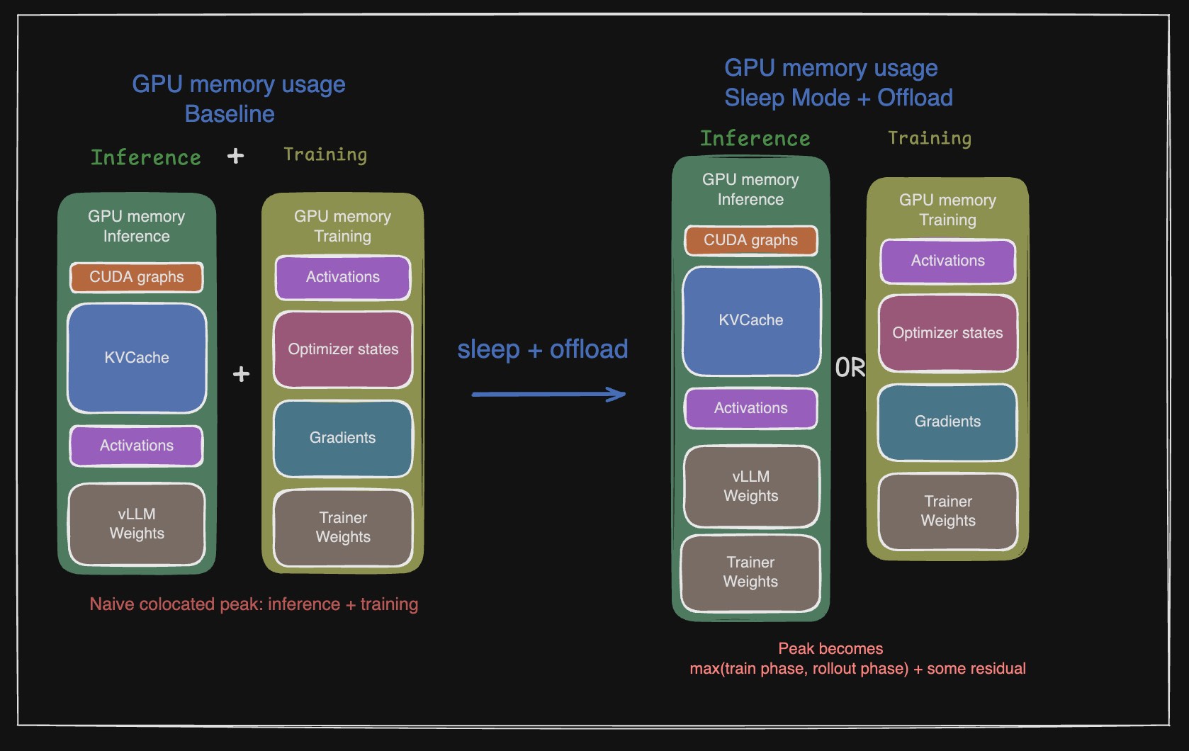The optimization is temporal: keep only the phase that is actively using VRAM.

The two big questions to answer here are

1. Can you spin up and shut down the inference engine quickly?
2. Can you offload the trainer components to CPU RAM quickly?

Inference Engine Startup/Shutdown

If you have ever interacted with vLLM, the startup time can take a few seconds to a few minutes. It goes through a whole lot of steps. We will take the example of Qwen3-32B on a B200 GPU for the time taken. Note that all these were benchmarked on a single GPU. If you do this on a multi-GPU system, profiling will take longer due to inter-GPU communication overhead.

• Weight loading The inference engine needs to load weights from disk to GPU memory. ~75s
• Profiling vLLM runs a dummy forward pass with the selected input sizes to estimate the activation memory requirement. This reduces the chance of OOMs and helps decide how many KV cache blocks can be allocated. You profile, understand memory requirements, and fail fast if it is not enough. ~32s
• CUDA Graph capture This is a very important step for performance. I have seen ~20-30% performance loss if you do not do this. ~9s
• KVCache allocation This is done to pre-allocate the KVCache memory so that we don’t have to allocate it during inference. This is pretty instantaneous.

The problem is that if you shut down and restart the server, you’re wasting at least a couple of minutes every step. If you want to do a large training run, this will be a significant portion of your total training time. If the generated tokens aren’t too many, this can potentially take more time than generation and the forward/backward pass. So you don’t want to do that, but you also don’t want to lose the memory advantages you get from freeing up the inference engine memory.

The middle ground is Sleep Mode from vLLM. What it does is discard/offload weights and KVCache, which is roughly the bulk of the inference engine memory anyway.

There are two sleep modes that vLLM exposes:

• Level 1: Offload model weights to CPU. Discard KVCache This took ~30s to sleep and ~0.6s to wake up in the benchmark I am referring to.
• Level 2: Discard model weights and KVCache. No CPU backup for the weights, though small model buffers may remain on CPU. This took ~0.24s to sleep and ~0.4s to wake up in the same benchmark.

For full finetuning RL workloads, we can choose to do Level 2 because the model weights are generally updated between sleep and wakeup, and we need the inference engine to have the latest weights anyway. Of course, wakeup has to be paired with loading/updating the weights before the next rollout. The exception is LoRA, where you want the shared base weights to stay resident (more on that later).

Chunked loss calculation

When you have a model like Qwen3-8B for GRPO, assume that you have a sequence length of 16K and a batch size of 4. Qwen3-8B has a vocab size of 151,936. In BF16, the memory usage looks like:

• Hidden States: bsz * hidden_size * seq_len = 16384 * 4096 * 4 * 2 bytes = 0.5 GiB
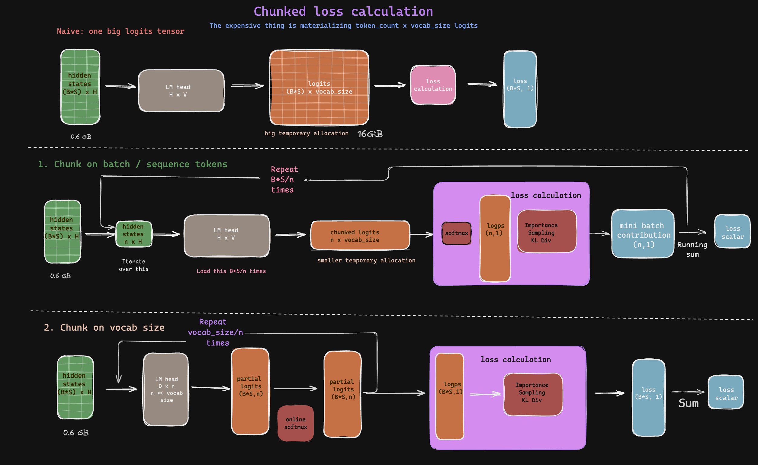
• Logits: bsz * vocab_size * seq_len = 16384 * 151936 * 4 * 2 bytes = 18.6 GiB

So if you materialise the logits, you’re going to pay a hefty price. The moral is to not materialise the logits. Hidden states are much easier on GPU memory, and we need to store or recompute them anyway because every subsequent layer works with the same shape/size.

\[\begin{aligned} \mu_G &= \frac{1}{G}\sum_{j=1}^{G} r_j \\ \sigma_G &= \sqrt{\frac{1}{G}\sum_{j=1}^{G}(r_j-\mu_G)^2} \\ \hat{A}_i &= \frac{r_i - \mu_G}{\sigma_G + \epsilon_{\text{std}}} \end{aligned}\] \[\mathcal{L}_{\mathrm{GRPO}}(\theta) = -\mathbb{E}_{q,\{o_i\}_{i=1}^{G}} \left[ \frac{1}{G}\sum_{i=1}^{G} \frac{1}{|o_i|} \sum_{t=1}^{|o_i|} \ell_{i,t}(\theta) \right]\] \[\ell_{i,t}(\theta) = \min\left( \rho_{i,t}(\theta)\hat{A}_i,\, \operatorname{clip}\left(\rho_{i,t}(\theta),1-\epsilon,1+\epsilon\right)\hat{A}_i \right) - \beta D_{\mathrm{KL}}\left( \pi_\theta(\cdot|s_{i,t}) \,\|\, \pi_{\mathrm{ref}}(\cdot|s_{i,t}) \right)\]

The loss is just a sum over the tokens of a sequence which is then aggregated over the group. So one token’s contribution to the loss is independent of other tokens in the same sequence once its log probability, advantage, and KL term are known. Instead of trying to materialise and calculate everything at once, what we can do is write a kernel which iterates over the tokens, calculates the loss for that token, and accumulates it. This way, we don’t have to materialise the logits and can keep memory usage low. We talked more about GPU architecture, how streaming output can be calculated, and how kernels can be useful in our previous blog The MathemaTricks behind Flash Attention.

There is one subtle point here. The exact KL term at a token position is a full-vocabulary expectation. But in practice, a lot of GRPO implementations use sampled-token approximations. For this post, the important bit is simple: we can often work with the generated token’s log probability instead of materialising the full vocabulary distribution for every token.

Pro Tip: Anytime there is an increase in dimension followed by a reduction, try to think if you can do the reduction in chunks. This can help you avoid materialising the intermediate result and save a lot of memory. You see the same trick in Flash Attention, Cut Cross Entropy, Fused MLP etc. But we also need to make sure our backward pass is appropriately dealt with and we save enough info for that.

# Simplified pseudocode: compute full-vocab logits only for a token chunk,
# then gather only the sampled-token logprobs needed for the policy ratio.
# In real PPO/GRPO code, old_logps are usually cached from rollout time
# or recomputed with the frozen behavior policy. This is shape-level pseudocode.
# hidden_states: (bsz*seq_len, hidden_dim)
# lm_head: (hidden_size, vocab_size)
def batched_chunked_loss(old_hidden_states, new_hidden_states, lm_head, sampled_tokens, advantages):
  total_loss = 0
  old_hidden_states = old_hidden_states.reshape(-1, mini_batch_size, hidden_dim)
  new_hidden_states = new_hidden_states.reshape(-1, mini_batch_size, hidden_dim)
  sampled_tokens = sampled_tokens.reshape(-1, mini_batch_size, 1)
  advantages = advantages.reshape(-1, mini_batch_size, 1)
  for old_mini_batch, new_mini_batch, mini_tokens, mini_advantages in zip(old_hidden_states, new_hidden_states, sampled_tokens, advantages):
    # Process each mini-batch
    # (mini_batch_size, hidden_dim) @ (hidden_dim, vocab_size) -> (mini_batch_size, vocab_size)
    old_mini_logits = old_mini_batch @ lm_head  # (mini_batch_size, vocab_size)
    old_mini_logps = F.log_softmax(old_mini_logits, dim=-1).gather(-1, mini_tokens)  # (mini_batch_size, 1)
    new_mini_logits = new_mini_batch @ lm_head  # (mini_batch_size, vocab_size)
    new_mini_logps = F.log_softmax(new_mini_logits, dim=-1).gather(-1, mini_tokens)  # (mini_batch_size, 1)
    log_ratio = new_mini_logps - old_mini_logps  # (mini_batch_size, 1)
    ratio = torch.exp(log_ratio)
    mini_batch_loss = clip(ratio, mini_advantages).sum()
    total_loss += mini_batch_loss
    pass
  return total_loss

Another optimization is to do the LM head multiplication in chunks where you split the LM head itself. But this would not directly resolve into any individual unit of the loss. So the accumulation would be slightly more involved. If you think about it, this is very similar to how we do Column Parallel vs Row Parallel in Tensor Parallelism. Also for how online softmax is implemented, please refer to the same in The MathemaTricks behind Flash Attention. The target token logit is easy. The annoying part is the denominator, because softmax needs to look at the full vocabulary. For the denominator, we need to look at all logits, but we need not store/persist them. They can be maintained via a running max and running sum while we iterate over the chunks.

# Simplified pseudocode.
# hidden_states: (bsz*seq_len, hidden_dim)
# lm_head: (hidden_size, vocab_size)
def chunked_lm_head_mul(old_hidden_states, new_hidden_states, lm_head, sampled_tokens, advantage):
  sampled_tokens = sampled_tokens.reshape(-1)
  def get_logps(hidden_states, lm_head, tokens):
    _, vocab_size = lm_head.shape
    N = hidden_states.shape[0] # bsz * seq_len: one per token per seq
    max_so_far = torch.full((N,), -float("inf"), device=device, dtype=torch.float32)
    sum_exp = torch.zeros((N,), device=device, dtype=torch.float32)
    sampled_token_logit = torch.empty((N,), device=device, dtype=torch.float32)
    for start_idx in range(0, vocab_size, chunk_size):
      end_idx = min(start_idx + chunk_size, vocab_size)
      chunk = lm_head[:, start_idx:end_idx] # (hidden_size, chunk_size)
      # Process chunk
      partial_logits = hidden_states @ chunk  # (bsz*seq_len, chunk_size)
      chunk_max = partial_logits.max(dim=-1).values
      next_max = torch.maximum(max_so_far, chunk_max)
      # If the max changes, rescale the old running sum to the new max before adding this chunk.
      sum_exp = sum_exp * torch.exp(max_so_far - next_max)
      sum_exp = sum_exp + torch.exp(partial_logits - next_max[:, None]).sum(dim=-1)
      max_so_far = next_max
      mask = (tokens >= start_idx) & (tokens < end_idx) # update for the chunk
      # each token in a batch/seq has its own vocab ID. they might or might not be in the current chunk
      # so we do a masked update
      sampled_token_logit[mask] = partial_logits[mask, tokens[mask] - start_idx]
    lse_vocab = max_so_far + torch.log(sum_exp)
    logp = sampled_token_logit - lse_vocab # log(exp(target_logit) / sum(exp(logits)))
    return logp
  
  old_logp = get_logps(old_hidden_states, lm_head, sampled_tokens) # (bsz, seq_len, 1)
  new_logp = get_logps(new_hidden_states, lm_head, sampled_tokens)
  log_ratio = new_logp - old_logp
  ratio = torch.exp(log_ratio)
  loss = clip(ratio, advantage).sum(dim=-1) # (bsz, seq_len)
  return loss

Chunked loss calculation

LoRA - Weight Sharing

By now you wouldn’t need a re-introduction to LoRA. Basically, instead of training full weights, you train an adapter (which is like a lego block) which keeps gradients and optimiser states in check, thus saving a lot of memory. For further details, read The Lore behind LoRA.

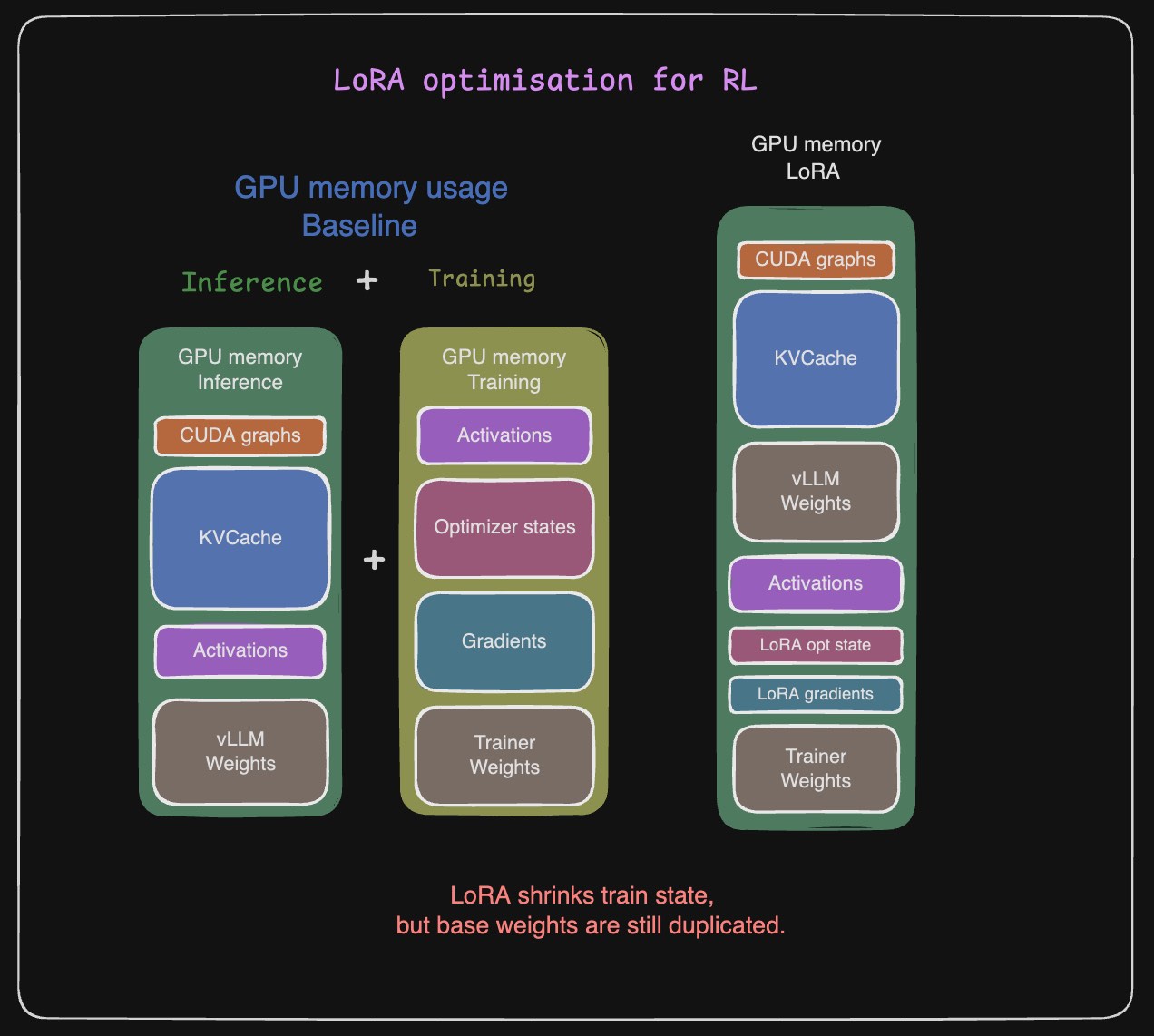
Because the base weights are frozen, for training, there is no need to track gradients or optimizer states for them, and the weights are left in inference-only mode. This is what vLLM also has anyway. So instead of storing two copies of the base weights, one for the trainer and one for the inference engine, we can load them once and reuse them. Conceptually, the trainer and vLLM hold two references to the same base-weight memory, and LoRA is loaded on top of that.

You can combine this optimization with sleep mode, but the only thing is you do not want to offload or discard the model weights because they are used by the trainer. Another side effect, which turns out to be an advantage, is that you save the time required to offload and onload weights. vLLM exposes a LoRA request mechanism to load the LoRA adapter for serving inference requests. One final optimization is to not store the LoRA adapter to disk and reload it from disk for the LoRA request, but load it in memory so that we skip the synchronization and copy path.

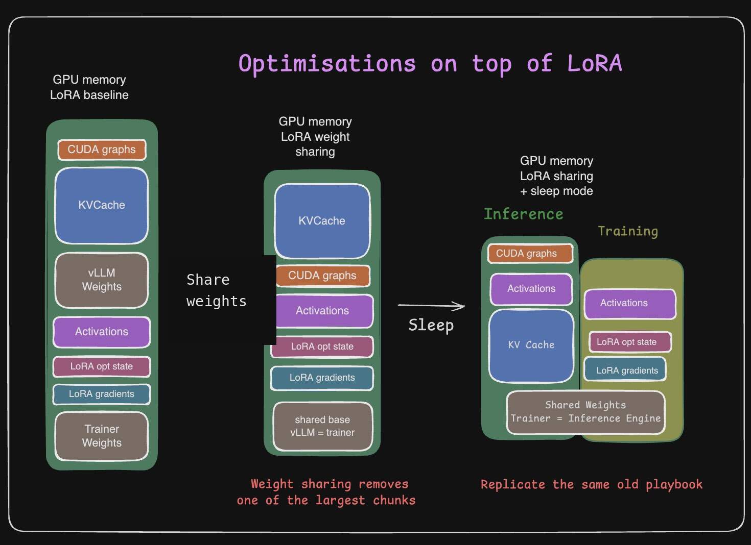When weights are shared, sleep mode should free transient inference state, not the shared base weights.

This can also be done for QLoRA as long as vLLM and the trainer agree on the quantized tensor storage layout. This can get trickier when kernels pack or reshape quantized tensors, especially for MoE models. So you have to be careful there.

The LoRA weight-sharing and sleep-mode style optimizations are a part of Unsloth, and it supports a lot of popular models like Qwen, Llama, Mistral, and Gemma, including their vision-language model families. All you need to do to enable this is

from unsloth import FastLanguageModel

model, tokenizer = FastLanguageModel.from_pretrained(
    model_name = "unsloth/Qwen3-4B",
    max_seq_length = 2048,
    dtype = None,
    load_in_4bit = False,
    fast_inference = True, # Enables weight sharing
    unsloth_vllm_standby = True, # Enables sleep mode optimisation
)

Async GRPO

Now flip the constraint. What would you do if you had enough office space and did not need to time-slot backend at night and frontend during the day? You would want to maximize utilization and get the work done as soon as possible. One possibility is that while backend engineers work on one feature, frontend engineers work on another, perhaps slightly older, feature. There is still overhead in syncing the codebase, but a few commits of lag may be manageable. Of course, you still need to sync everyone to the same state every once in a while so the drift does not become too large.

Assuming that you are not GPU poor and have multiple GPUs to play around with for GRPO, ask yourself the same question again. What is the inference GPU doing when the trainer is updating? And what is the trainer GPU doing when inference engines are generating rollouts? And of course, there is a sync phase happening at the boundary as well. They’re just idle. In general, synchronous and sequential is preferred because it is mathematically cleaner. But it has been observed multiple times that even when the weights are nominally the same, kernel changes, batch-size changes, precision choices, and inference-engine differences can create a drift between the logits or completions generated by the trainer and those generated by the inference engine. People tend to use importance sampling and other correction methods to handle this. But if you are going that far anyway, why not accept that there is a slight drift and not enforce strictly sequential generation/rollout and training?

This is exactly what Async GRPO does, where the inference engine on one GPU generates rollouts for the second batch while the trainer is forward passing through the first batch. This means that the inference engine is behind by a step or two when it comes to the weights. But because we do trust-region-style clipping and other stabilizers, a couple of steps of lag may be tolerable with importance sampling.

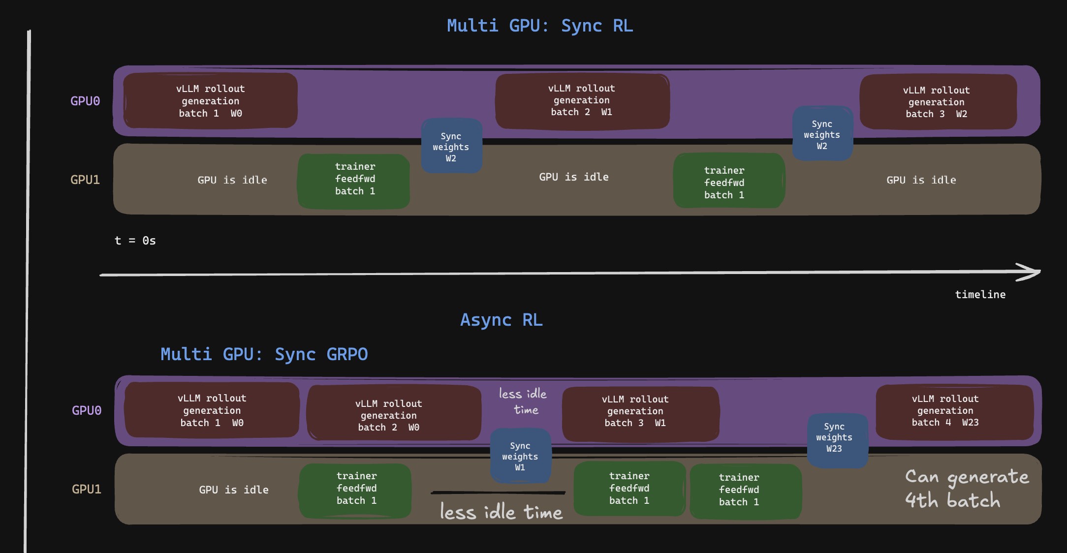Async GRPO overlaps rollout and training, accepting small policy lag for higher utilization.

You can go even further and make sure that the weight sync doesn’t pause rollout generation for too long. As in, while tokens are being generated, you update the weights one chunk at a time. So there is a possibility that within a single completion, some tokens are generated using older weights and some are generated using newer weights. The INTELLECT-3 technical report from Prime Intellect mentions that without in-flight weight updating, their RL step time increased by more than 2x. But this is a choice with a real tradeoff. If the KV cache was produced using older weights, then updating weights mid-completion means you are no longer dealing with a clean single-policy rollout. You either track the actual behavior logprobs/version closely, or you accept the approximation for the utilization win.

One needs to be careful to make sure that we are not overdoing these optimizations where there is a mismatch between the trainer and inference engine. If the difference becomes too high, then we are essentially doing off-policy learning instead of on-policy learning, which is less robust.

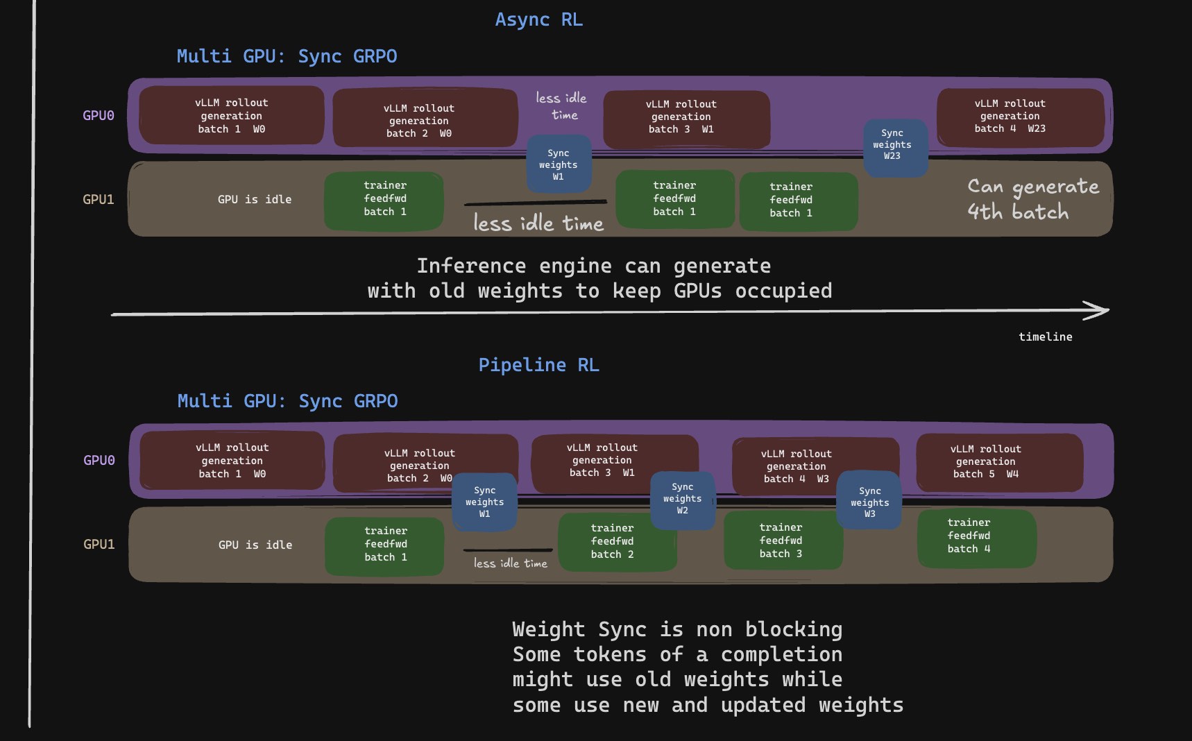Pipeline GRPO lets rollout continue while newer weights arrive, trading exact synchronization for utilization.

The advantages may be more pronounced for larger-scale model training, especially across multiple nodes where weight sync time is bound by network speed and can bottleneck the entire training. For intra-node communication on PCIe or NVLink, especially for small-scale model training, you might get away without these optimizations, but they are still worth measuring.

Delta weight sync

So when working with codebase updates, do you ship the entire codebase every night between the teams and wait while syncing is happening? You’d invent something like Git and just share the patches or diffs. Assuming that the delta is smaller than the object itself, this is well worth the trade off. But of course, you need some bookkeeping on what changes are being made, where they are, and how to apply them correctly.

There is also a reason for exploring the possibility of compressing the weight updates. Typically, when you do mixed-precision training, any change that is less than half the local spacing of the data type will be rounded away. For example, in BF16 you have

    _        _ _ _ _ _ _ _ _      _ _ _ _ _ _ _ _
Sign bit     8 exponent bits      7 mantissa bits

So between any two consecutive powers of 2, we have 7 bits of precision, aka 128 intervals to play with. For a weight of magnitude |w|, the spacing is approximately |w|/128 within that exponent range. Anything less than roughly half that spacing (so about |w|/256) will round away. It’s like doing 10^3 += 0.1 but you can only represent whole numbers. For this to make any change in the value, it needs to be at least 0.5 so that rounding will carry it over to the next representable value (a whole number in the example, BF16 in reality).

Typically, the weights in LLMs are around the scale $1e^{-2}$. So the BF16 spacing around that value is approximately $1e^{-2}/128 \approx 7.8e^{-5}$, and anything below half of that, roughly $4e^{-5}$, gets rounded away. RL learning rates are usually tiny, often around $3e^{-6}$. Pair that with norm-based gradient clipping and the small gradients typical of RL, and the effective optimizer update per step can comfortably sit below that $\approx 4e^{-5}$ threshold. When it does, the stored BF16 value simply does not move. This does not mean the optimizer state did not change. If you maintain FP32 master weights or optimizer states, those can still accumulate the update across steps until it eventually crosses the threshold. The point is that the BF16 copy you sync/serve may remain bit-identical between two consecutive steps.

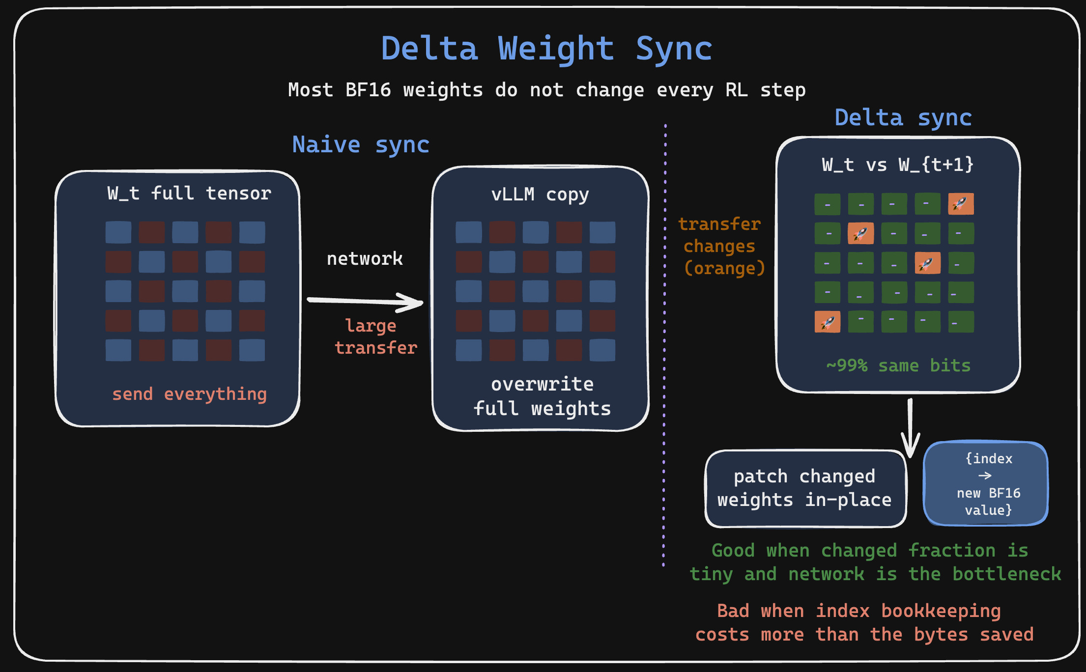
It is also empirically observed that approximately 99% of stored BF16 weights can remain bit-identical between consecutive RL optimizer steps in some mixed-precision RL training settings with lower learning rates (and rarely below 98% in the worst case). So one thing you can do is, instead of sharing the entire weight tensor over the network, identify the specific positions where updates have actually changed the stored BF16 value and share only those values. If the updates are dense or the model is small, this bookkeeping can cost more, especially on high-speed interconnects like PCIe or NVLink. But over the network for large-scale models, the bookkeeping cost can be amortized and save a lot of time. You can read more in HuggingFace’s Delta Weight Sync writeup.

So how do you take advantage of this? Instead of sharing the entire weight tensor, we might as well just share the “delta” (in literal and analogy sense). Instead of sharing an entire tensor of shape (m, n), you share a map {index: new_value} where index is the flattened position of a value that actually changed. Now here’s a subtlety worth pausing on: how big does that index have to be? A single weight matrix can have hundreds of millions of elements, so an int8 or even int16 index (max 32,767) cannot address them. In practice you need an int32 index, which is 4 bytes, paired with the 2-byte BF16 value. So you are paying ~6 bytes per changed value, roughly 3x the bare value. That sounds wasteful until you remember you’re only shipping ~1% of the elements. Of course, this also assumes that the inference engine can hot-swap particular weights and indices on the fly, either through native support or a worker extension.

Delta weight sync in action

TLDR

• LLM on-policy RL needs inference engines to be efficient.
• On colocated setups where trainer and inference share the same GPUs, sleep mode and optimiser state offload can save a lot of memory.
• On distributed setups, going slightly off-policy (generation weights are a few steps behind) with asynchronous training and pipelining reduces GPU idle time and speeds up training.
• A lot of synced BF16 weights can remain bit-identical with low LR (~3e-6) in RL. Sharing only the updated values and indices can save a lot of network bandwidth.

Conclusion

Anytime ML researchers come up with a new algorithm, function, or mechanism, ML engineers have to sit and optimise the system to squeeze out every last bit of performance. Sometimes model-hardware co-design is done to avoid a lack of cohesion. But when doing something novel, you cannot possibly foresee and optimise for every scenario. After every new research innovation, there are usually systems optimisations that become visible if you look at things from a utilization standpoint and try to eliminate gaps. This is one such example of making things faster and more efficient. With that, as promised, I present you the systems side of LLM-RL. I’ll take your leave. Happy learning! Stay curious…

References

• Reinforcement Learning for LLMs (the predecessor to this post)
• vLLM and SGLang inference engines
• vLLM Sleep Mode
• vLLM LoRA serving
• Qwen3-8B config
• The MathemaTricks behind Flash Attention
• Cut Cross Entropy
• Understanding Multi-GPU Parallelism Paradigms
• The Lore behind LoRA
• Your Efficient RL Framework Secretly Brings You Off-Policy RL Training
• INTELLECT-3 Technical Report
• Shipping a Trillion Parameters With a Hub Bucket: Delta Weight Sync in TRL